Managing Large Data Amounts when using Techila Distributed Computing Engine in Google Cloud Platform Marketplace

1. Introduction

Techila Distributed Computing Engine is a big computing solution that supports interactive high-performance computing. The solution is available as a pay-as-you-go solution in Google cloud platform marketplace (GCP Marketplace). It is also available with an enterprise license that can be cost-efficient in sustained use.

Many computational workloads use or produce data. In some cases the volumes of data can be significant. This document is intended for End-Users and IT support staff and describes how to efficiently manage large amounts of data when using Techila Distributed Computing Engine Advanced Edition in Google Cloud Platform Marketplace by using Google Cloud Storage.

The structure of this document is as follows:

The Data chapter contains an overview of different aspects of data, what needs to be done in order to make the data accessible during computational Project and introduces some popular options for transferring data when using TDCE.

The Examples chapter describes how to use the Google Cloud SDK to transfer files when processing computations in TDCE. This chapter also contains an overview of the process needed in order to configure the Google Cloud SDK on the End-User’s computer, which will allow transferring files using Google buckets.

Please note that in the scope of this document, data is thought to consist of either local data files or information stored in workspace variables. This document does not cover using databases in Techila Distributed Computing Engine.

2. Data

Data used by applications might be general in nature, for example, consisting of a large number of files containing text, audio or image data.

When working with an application, the data might be stored using programming language specific file formats. Some examples of commonly used programming language specific file formats include MAT files when using MATLAB or .RData and .rds when using R.

Lastly, the data might be more temporary in nature and only exist as workspace variables in the application that you are working with.

Regardless of the data formatting differences, there are some common aspects they all share: the location and size of the data. These properties become very relevant when switching from a local application to a distributed version.

2.1. Data Location

When running code on your local computer that accesses local data files, you typically do not need pay any special considerations about how to access the data. Alternatively, your data could be located on a network file system that has been designed to be used with computational workloads. In either case, this means that the location of the data is quite well suited for computational purposes, meaning no additional effort needs to be done in order to make the data accessible when running your application.

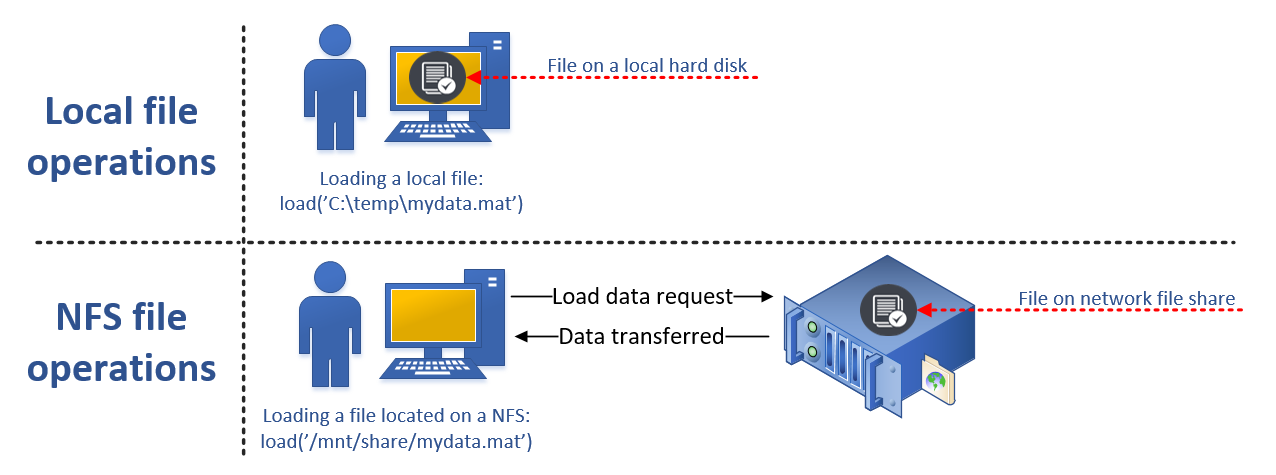
Figure 1. Local applications are typically able to access local data resources with minimal effort.

However, when switching from a local computing environment to a distributed computing environment, the computational processes will no longer run on your computer. This means that some thought needs to be given to the location of the data and what needs to be done in order to make it accessible when computations are running in the distributed computing environment.

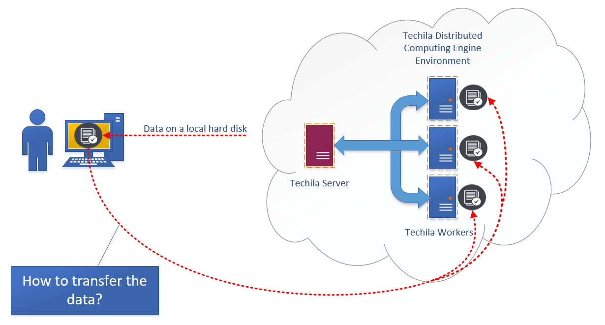
Figure 2. When using Techila Distributed Computing Engine, data needs to be transferred to the Techila Workers so it can be accessed during computations.

Typically this means that the data needs to be transferred from its current location to a location that can be accessed when processing the computational code on Techila Workers. More information on available options can be found in Data Transfer Options.

3. Data Transfer Options

Depending on the amount of data, there are two possible options that can be used:

Bundles
Google Cloud Storage

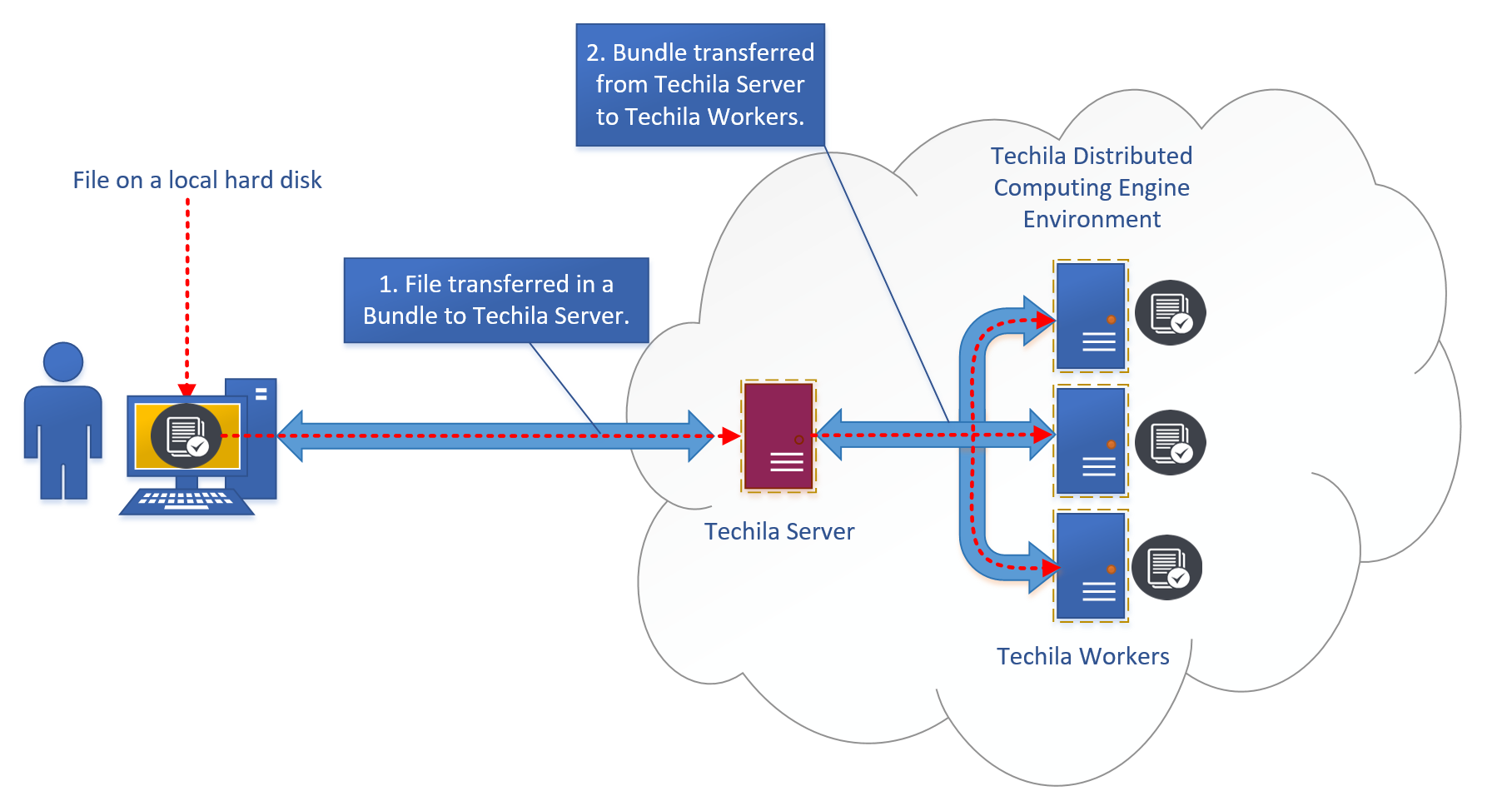
3.1. Bundles

Bundles are the automatic solution that Techila Distributed Computing Engine uses for transferring data. This is a built-in technology that provides automatic versioning and supports automatic optimization of data transfer between the user and the system and within the system. Bundles provide an easy-to-use and convenient way to transfer small data amounts.

There is no hard limit on what constitutes as "small", as everything depends on the properties of the computational problem, or more specifically, how much computational work will be done using the data. The higher the amount of computational work done per transferred byte, the less impact non-optimal data transfer routines will have on overall performance. More general information about distributed computing economics can be found in this technical report by Microsoft.

As a rule of thumb, Bundles should only be used when the data amount is below 1 GB. When the amount of data is larger than 1 GB, using Google Cloud Storage typically provides better performance. When the Bundle-based data management that uses the Techila Server as a gateway becomes a bottleneck, an interesting solution can be a so-called bucket that is a Google Cloud Storage service.

Figure 3. Flow of data when using Bundles.

For more information on how to transfer data files using Bundles, please see the programming language specific examples in the how-to guides. Pointers to some commonly used programming language examples are included below for convenience:

When working with a set of input files that you want to process separately, the Job Input Files feature provides an alternative method for transferring files. Pointers to some commonly used programming language examples are included below for convenience:

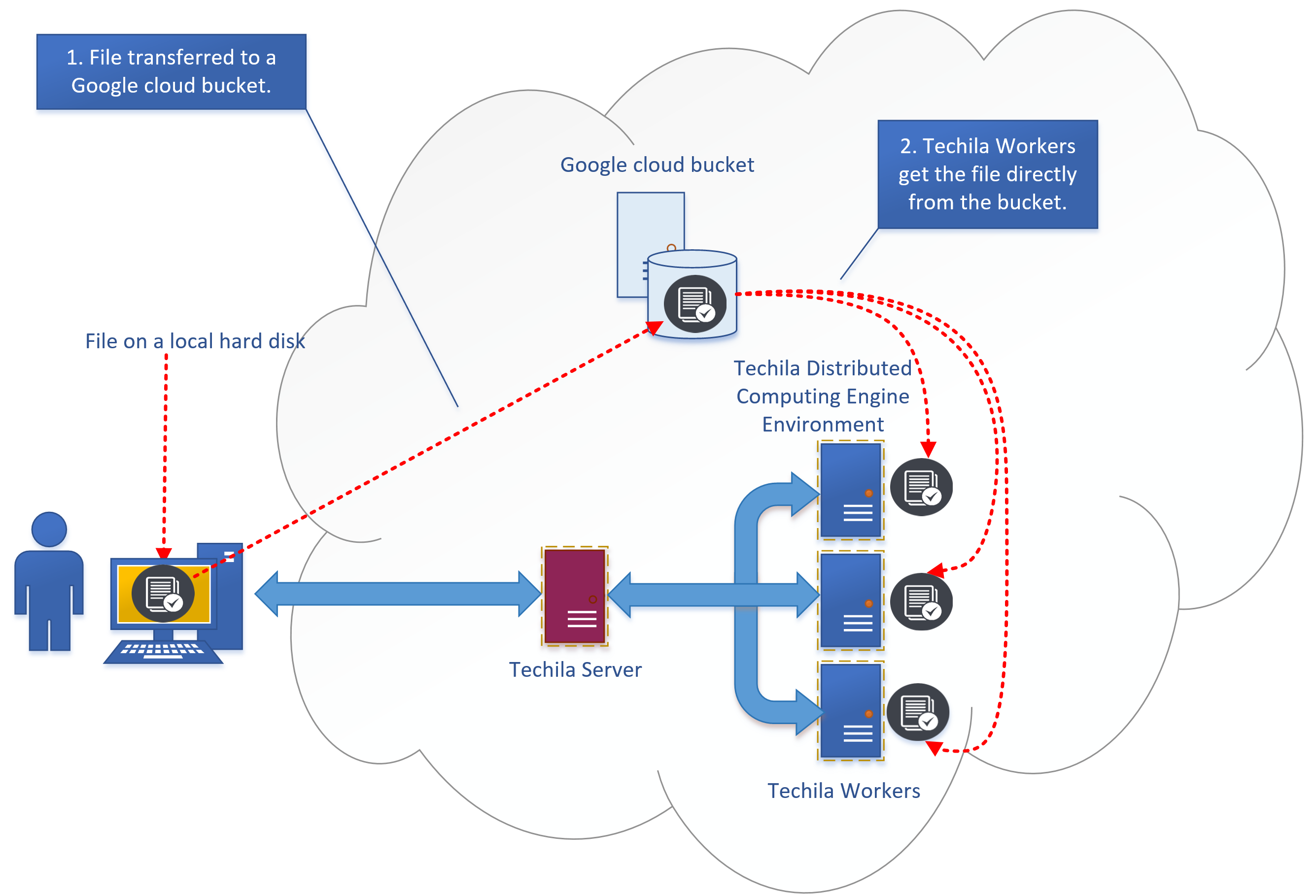
3.2. Google Cloud Storage

Google Cloud Storage is an online file storage service for storing and accessing data on Google Cloud Platform infrastructure. When working with large data amounts, Google Cloud Storage provides a fast and scalable way to transfer data. Google Cloud Storage can be used to transfer data in both directions, meaning it can be used to transfer input data from your computer to TDCE and/or result data from TDCE to back your computer. Alternatively, you can of course leave the result data stored in Google Cloud Storage, if you do not want to post-process it on your computer.

Two popular methods for transferring data between a computer and a buckets are:

gsutil - Command line interface for transferring files. Works on Windows and Linux.
gcsfuse - Method for mounting a bucket as a file system. Works on Linux.

3.2.1. gsutil

In order for an End-User to access Google Cloud Storage, the End-User’s computer will need to have the Google Cloud SDK installed and configured to use the desired bucket. Additionally, code logic will need to be added to the application so it can perform the necessary file transfers when it will be executed in TDCE. The file transfers can be done by using the gsutil Command Line Interface (CLI) command included in the Google Cloud SDK. The gsutil command provides many useful commands for managing cloud data, most notably the cp command, which allows you to copy data between a local file system and the cloud bucket.

Figure 4. Flow of data when using buckets.

For reference, a couple of simple examples are included below. Let’s assume that you have created a bucket named my-cloud-data and want to transfer a file called my_local_file.txt from your computer to the bucket. This could be done with the following command:

gsutil cp my_local_file.txt gs://my-cloud-data

Respectively, if we assume that you have a file called my_cloud_data.txt stored in bucket my-cloud-data, you could transfer it from the cloud to your computer (to the current working directory) with the following command:

gsutil cp gs://my-cloud-data/my_cloud_data.txt .

Multiple files can be transferred by defining a suitable expression. For example the following syntax could be used to transfer all MAT files from the current working directory to the bucket. The -m option in the command parallelizes the transfer process, which typically improves performance when transferring a large number of files.

gsutil -m cp *.mat gs://my-cloud-data

The gsutil commands can also be executed from any programming language you are using by performing a system command call. When using MATLAB or R, the syntax is identical in both languages and is shown below for reference.

cmd = 'gsutil cp image1.png gs://my-cloud-data'
system(cmd)

The exact syntaxes used to execute system commands for other programming languages might be slightly different, but the actual gsutil command will follow the same principle regardless of what programming language you are using.

Another option for transferring files is the rsync command, which can be used to synchronize content of two buckets/directories.

Please note that when using Techila Distributed Computing Engine Advanced Edition in Google Cloud Platform Marketplace, The Google Cloud SDK is automatically installed on all Techila Workers, meaning you can execute gsutil cp commands on Techila Workers to transfer files to and from buckets located in the same GCP project.

Example: MATLAB application that processes 1000 independent images.

Consider a situation where you have a MATLAB application that is processing 1000 independent images using the following for loop.

function main()
  for x = 1:1000
    % Load image.
    data = imread(['image_' num2str(x) '.png']);

    % Some hypothetical, computationally intensive operation on data.
    res(x) = hypo_op(data);
  end
end

Each iteration in the above application only needs access to one file, as determined by the loop counter index. This means that when pushing the above workload to Techila Distributed Computing Engine using cloudfor, each iteration will only need access to the one, specific image that is being processed. The below code snippet shows how the data transfers could be handled using gsutil cp command.

function main()
  % Run gsutil cp command locally to transfer image files from your computer
  % to a bucket called 'my-cloud-data'.
  cmd = 'gsutil -m cp image_*.png gs://my-cloud-data';
  system(cmd);

  cloudfor x = 1:1000
    if isdeployed
        % Transfer the needed file from the bucket to the Techila Worker
        cmd2 = ['gsutil cp gs://my-cloud-data/image_' num2str(x) '.png .']
        system(cmd2);

        % Load image.
        data = imread(['image_' num2str(x) '.png']);
        % Some hypothetical, computationally intensive operation on data
        % Assuming the result data is relatively small, we can simply store
        % the result in the 'res' array, which will be automatically returned
        % to the End-User's MATLAB session.
        res(x) = hypo_op(data);
    end
  cloudend
end

3.2.2. gcsfuse

gcsfuse can be used to mount a bucket on Techila Workers as a filesystem. After mounting, files can be accessed using similar syntaxes that you would use to access local files. Please note however, that writing files to and reading files from GCS has a much higher latency than using a local file system.

Never mount the bucket under the current working directory ('.') or the home directory during the Job as these directories will always be automatically cleaned at the end of the Job, meaning all bucket data would also be deleted.

You can use the following approach to mount a bucket on a Techila Worker.

function main()

bucketname = 'my-cloud-bucket'

% NOTE! Never mount under the current working directory OR under home
% directory, because they will be deleted at the end of the Job.
mntpoint = '/tmp/test'; % Mountpoint. To be safe, always mount somewhere under /tmp/.

disp(['Mounting bucket ' bucketname ' using gcsfuse on Techila Workers'])
disp(['Bucket will be mounted to: ' mntpoint])

% Beginning of the cloudfor-block. This will mount the bucket on Techila Workers.
cloudfor idx=1:10
%cloudfor('stepsperjob',1)
%peach('ProjectParameters',{{'techila_multithreading_project','true'}})
%cloudfor('mfilename','gcsfusemount.m')
if isdeployed
    setenv('MATLAB_SHELL', '/bin/sh')
    mkdir(mntpoint) % Create the mountpoint directory
    [a{idx},b{idx}] = system(['gcsfuse --implicit-dirs ' bucketname ' ' mntpoint]) % Mount it
    [c{idx},d{idx}] = system(['dir ' mntpoint]) % Get file list for debugging purposes
end
cloudend % End of the cloudfor-block

% At this point the bucket is mounted on Techila Workers. You can now create a computational project where you access the files.

% Beginning of the cloudfor-block. During these Jobs, you can access the bucket file contents from the mount point.
cloudfor idx=1:100
if isdeployed
    setenv('MATLAB_SHELL', '/bin/sh')
    load([mntpoint '/' 'some_arbitrarary_file_in_bucket.mat']) % Load data from the bucket
    % Code commands for using the data from the file could be added here.
end
cloudend % End of the cloudfor-block
end

4. Requirements

In order to transfer files between your computer and the Cloud Storage bucket, you will need to install the Google Cloud SDK on your computer. Additionally, you will need to create a bucket where the files will be stored.

Please see the process below for steps on how to create a set up and test Google Cloud SDK on your computer.

Process

Download, install and initialize the Google Cloud SDK on your computer. Instructions for installation can be found at the link shown below.

https://cloud.google.com/sdk/

Note! When configuring the Google Cloud SDK, make sure that you set it up to use the same GCP project as you are using for your TDCE environment. It is also recommended to configure the Google Cloud SDK to use the same Region and Zone as you are using for your TDCE deployment.
Using your web browser, navigate to the Google Cloud Console. Select the correct project (the same one you are using for your TDCE environment and Google Cloud SDK) and enter create bucket in the search box and click on the matching search result.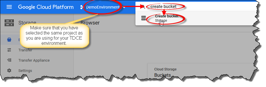
Click the Create bucket button to create a bucket that will be used to store the data.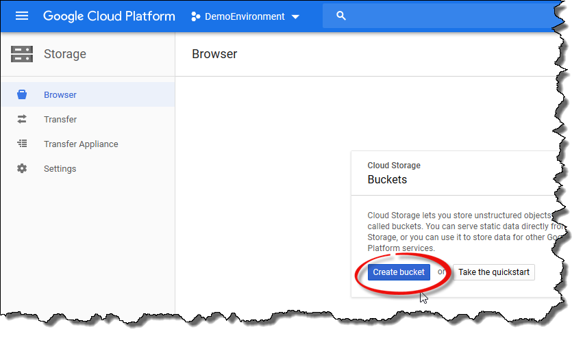
Specify a unique name for the bucket and choose either Multi-Regional or Regional as the default storage class. Set the Location to match your TDCE deployment location. Please note that depending on which storage class you chose, the appearance of the Location drop-down menu will be different. Finally, click the Create button to create the bucket.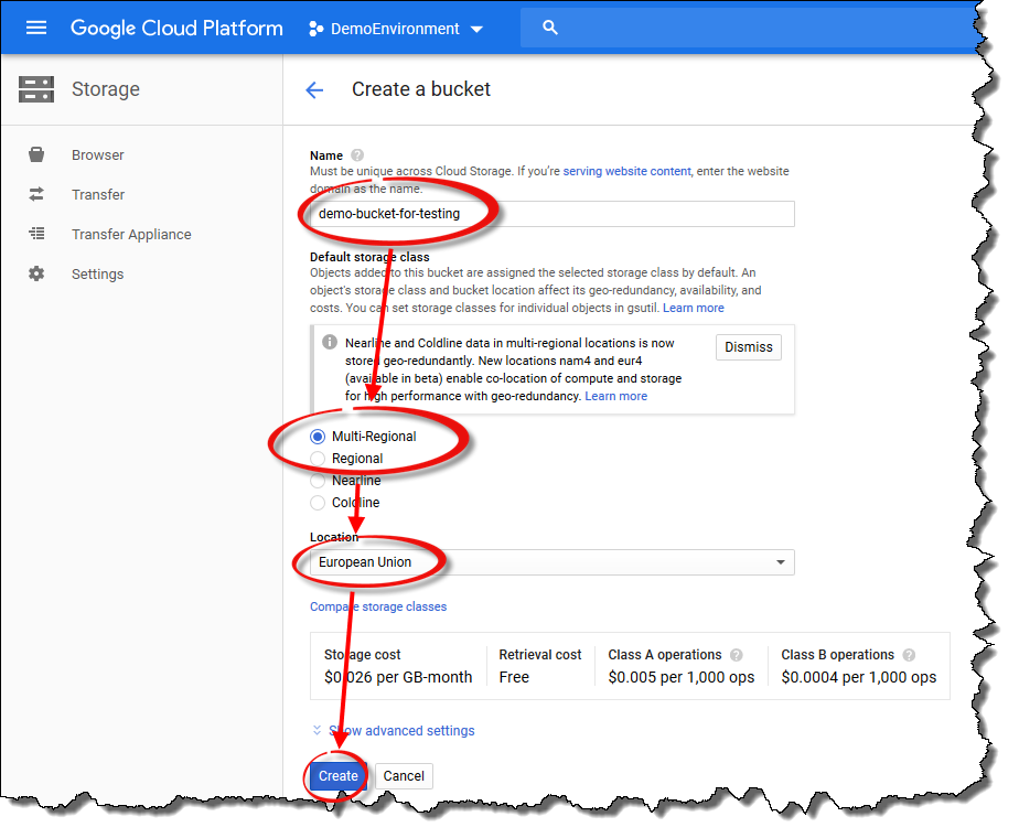
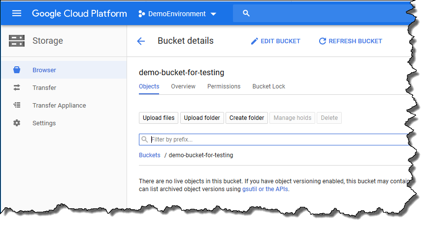
After creating the bucket, your view should resemble the one shown below. At this point, there are no files in the bucket.
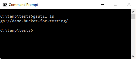
Next, test that gsutil works by executing the following command in your command prompt / terminal. If everything works ok, the bucket you just created should be displayed in the command’s output.
```
gsutil ls
```
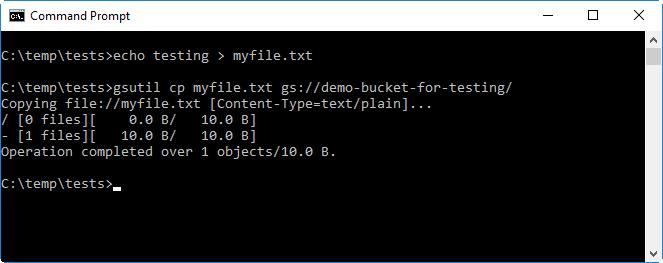
Next, check that you can write files to the bucket. To do this, create a simple text file called myfile.txt, save it to the current working directory and upload it to the bucket. The file can be uploaded using the gsutil cp myfile.txt gs://<your-bucket> command, where <your-bucket> needs to be replaced with the name of the bucket you created in the previous steps.

The example syntax below shows how the file can be created and then uploaded to a bucket named demo-bucket-for-testing.
```
type testing > myfile.txt
gsutil cp myfile.txt gs://demo-bucket-for-testing/
```
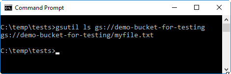
After uploading the file, check that it is in the bucket by using the gsutil ls <your-bucket> command, where <your-bucket> needs to be replaced with the name of the bucket you created in the previous steps.

The example syntax shows below how the command syntax would look like if the name of the bucket is demo-bucket-for-testing.
```
gsutil ls gs://demo-bucket-for-testing
```
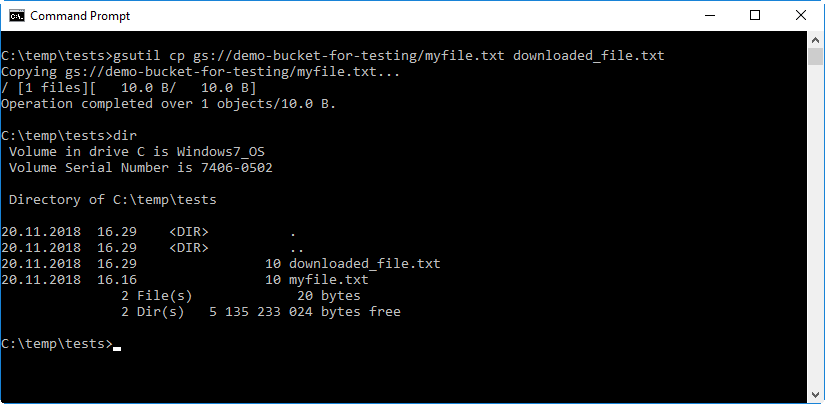
Finally, verify that you can download files from the bucket by using the gsutil cp command.

The example syntax shows below how the command syntax would look like if the name of the bucket is demo-bucket-for-testing. The last parameter in the syntax defines that the file should be saved on a new name downloaded_file.txt to avoid confusing it with the existing local file.
```
gsutil cp gs://demo-bucket-for-testing/myfile.txt downloaded_file.txt
```
You can also check the bucket contents from the GCP console. To do this, click the Refresh bucket icon in the GCP console view.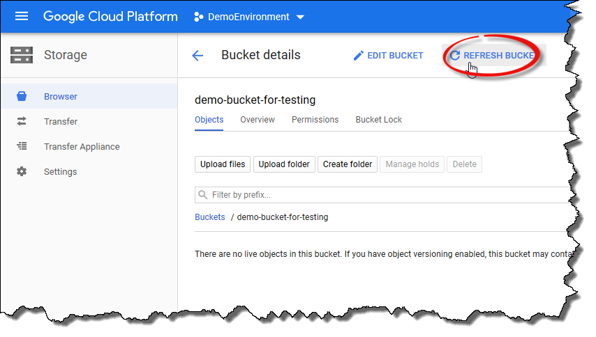

After the view has been refreshed, the file myfile.txt should be visible in the file listing.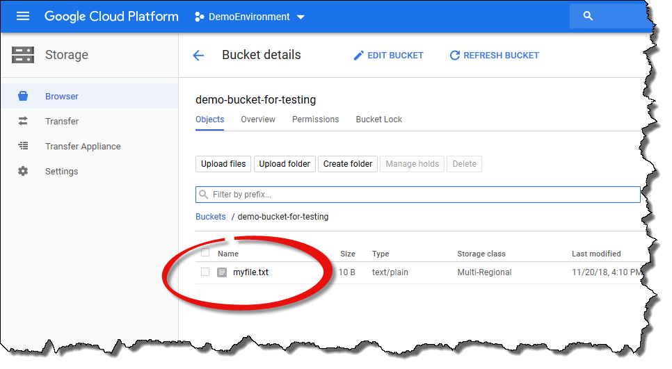
You can now transfer files between your computer and the Google Cloud Storage. The Techila Workers will automatically have the necessary permissions to access data from the bucket, as long it is located in the same GCP project with the TDCE deployment. You can now continue with running the examples.

5. Examples

This Chapter contains examples on how to use Google Cloud Storage to transfer data when using Techila Distributed Computing Engine Advanced Edition in Google Cloud Platform Marketplace. Please note that in order to run the examples, you will first need to do the configuration steps listed in Requirements.

There is one example per programming language. This example will show how to use the cloud bucket to transfer files during a computational Project.

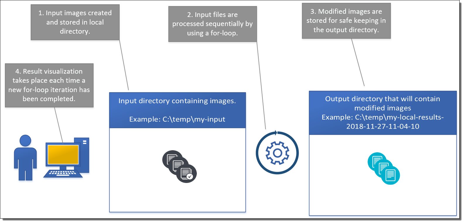
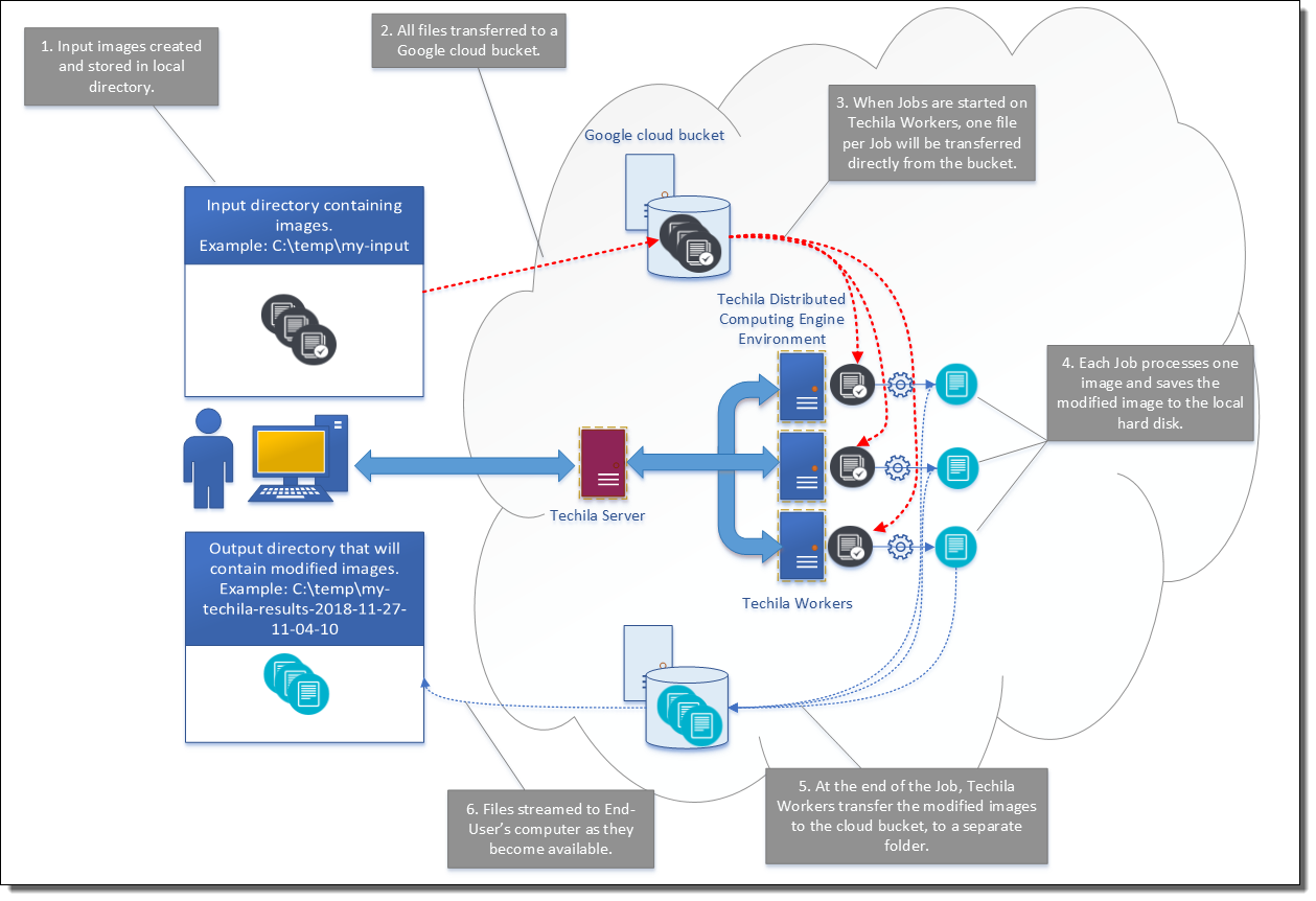
The flow of operations is the same in all programming languages and is illustrated in the images below.

Figure 5. Flow of operations in the local version.

Figure 6. Flow of operations in the TDCE version.

5.1. MATLAB - gsutil File Transfers

The MATLAB example in this Chapter shows how a locally executable data-intensive application can be converted into an efficient distributed version that will be executed in TDCE by using gsutil to transfer data.

5.1.1. Local Version

The local version will start by generating a set of random images and storing them to the input directory. After generating the images, a for loop is used to process the images by using a computationally intensive operation. In this example, this part of the application is represented by a one minute while loop that simply generates random numbers. After this, the modified image is stored to the output directory and some data visualization is done based on the modified image data.

The code for the local application is shown below:

function main_local()
  % Local version that processed images locally.

  % Number of images to process.
  img_count = 100;

  % Folder names used in the computations.
  ts = datestr(now,'yyyy-mm-dd-HH-MM-SS');
  tdir = 'my-input';
  resdir = ['my-local-results-' ts];
  prefix = 'my_image_';

  %% Data generation part.
  if exist(tdir,'dir') ~= 7
      mkdir(tdir);
  end
  mkdir(resdir);

  % Create new image set.
  % Start by removing old images.
  disp('Deleting old images')
  delete([tdir filesep '*.png'])
  disp('Done deleting old images')

  % Create new images.
  im_start = tic();
  disp('Creating random images..')
  for x = 1:img_count
      if mod(x,10) == 0
        disp(['Creating image ' num2str(x) ' of ' num2str(img_count) ...
           '. Estimated time remaining: ' num2str((img_count - x) *   toc(im_start)/x)...
           ' seconds.'])
      end
      rndata = randi(255, 1000, 'uint8');
      imwrite(rndata, [tdir filesep prefix num2str(x) '.png'])
  end
  disp('Done creating images..')

  %% Computational part.

  % Create an array for the results.
  res = zeros(1,img_count);

  % Result visualization init.
  figure
  h = histogram(NaN);
  [~,BinEdges] = histcounts(NaN,100);
  BinLimits = [min(BinEdges),max(BinEdges)];
  h.Data= NaN;
  h.BinEdges= BinEdges;
  h.BinLimits= BinLimits;
  title('Intensity average values')
  ylabel('Count of intensity value')
  xlabel('Intensity value')
  % Process images using a 'for' loop
  for x = 1:img_count

      disp(['Processing image ' num2str(x) ' of ' num2str(img_count)])
      % Load hypothetical image.
      data = imread([tdir filesep prefix num2str(x) '.png']);

      % Specify where the modified data will be stored.
      res_name = [resdir filesep 'my_result_image_' num2str(x) '.png'];

      % Some computationally intensive operation on data.
      % Assuming the result data is relatively small, we can simply store
      % the result in the 'res' array, which will be automatically returned
      % to the End-User's MATLAB session.
      res(x) = hypo_op(data, res_name);

      % Update the histogram to do some visualization on the result data.
      data_new = res(find(res~=0));
      updategraph(h, data_new)
  end
end

The code used to update the graph shown below for reference.

function updategraph(h, data_new)
% Copyright 2019 Techila Technologies Ltd.
% Function used to update the histogram plot with new data.
[~, be] = histcounts(data_new, 100);
bl = [min(be), max(be)];
h.Data = data_new;
h.BinEdges = be;
h.BinLimits = bl;

% Allow graph some time to update changes.
pause(0.01)
end

5.1.2. Distributed Version

The distributed version will start similarly as the local version, generating a set of random images and storing them to the input directory.

After generating the images, the images will be transferred to a bucket using the gsutil cp command.

After transferring the images to the bucket, a cloudfor loop is used to process the images on Techila Workers. Each Job will start by retrieving one image from the bucket and storing it in the temporary working directory on the Techila Worker. After the input file has been transferred, the same computationally intensive operation will be executed as in the local version. When the operations have been completed, the modified image will be stored on the Techila Workers hard disk from where it will be transferred to the bucket using a gsutil cp command. After the modified image has been transferred, the Job will be completed.

The modified image files will be automatically transferred to the End-User’s computer from the bucket by using the gsutil rsync command located in the callback function (cbfun.m).

The main TDCE function is shown below for reference.

function main_techila()
  % Copyright 2019 Techila Technologies Ltd.
  % Distributed version that uses cloud buckets for data transfers in TDCE.
  disp('Starting process...')

  % Name of bucket used to transfer images.
  % Change this to match the name of your bucket.
  bucket = 'demo-bucket-test';

  % Number of images to process.
  img_count = 100;

  % Bucket and folder information used in the computatinos
  bucket_folder = datestr(now,'yyyy-mm-dd-HH-MM-SS');
  tdir = 'my_tec_data';
  resdir = ['my_techila_results_' bucket_folder];
  prefix = 'my_image_';
  input_bucket_folder = 'my-input';
  output_bucket_folder = ['my-output-' bucket_folder];

  %% Data generation part.
  if exist(tdir,'dir') ~= 7
      mkdir(tdir);
  end
  mkdir(resdir);

  % Create new image set.

  % Start by removing old images
  disp('Deleting old images')
  delete([tdir filesep '*.png'])
  disp('Done deleting old images')

  % Create new images.
  im_start = tic();
  disp('Creating random images..')

  for x = 1:img_count
      if mod(x,10) == 0
        disp(['Creating image ' num2str(x) ' of ' num2str(img_count) ...
           '. Estimated time remaining: ' num2str((img_count - x) *   toc(im_start)/x)...
           ' seconds.'])
      end
      rndata = randi(255, 1000, 'uint8');
      imwrite(rndata, [tdir filesep prefix num2str(x) '.png'])
  end
  disp('Done creating images..')

  %% Computational part.

  % result array
  res = zeros(1,img_count);

  % result visualization
  figure
  h = histogram(NaN);
  [~,BinEdges] = histcounts(NaN,100);
  BinLimits = [min(BinEdges),max(BinEdges)];
  h.Data= NaN;
  h.BinEdges= BinEdges;
  h.BinLimits= BinLimits;
  title('Intensity average values')
  ylabel('Count of intensity value')
  xlabel('Intensity value')

  % Upload images to the Google bucket.

  cmd = ['gsutil -m cp ' tdir filesep prefix '*.png gs://' bucket '/' input_bucket_folder '/' ];
  disp(['Uploading images to the Google bucket using command: ' cmd])
  [stat, cmdout] = system(cmd);

  if stat ~= 0
      disp(['Something went wrong. Status code: ' num2str(stat)])
      error(cmdout)
  else
      disp('Done uploading images')
  end
  % Create a timer that will be used to throttle how often gsutil commands
  % are executed in 'cbfun' function.
  global dtimer;
  dtimer = tic();

  % Cloudfor callback parameters explained:
  %
  %cloudfor('callback','cbfun(res_name, bucket, output_bucket_folder)')
  % = Defines that 'cbfun' will be used as a callback function. This
  % function will be automatically executed whenever new results are
  % available. In this example, 'cbfun' will download result files from the
  % bucket to the End-User's computer.
  %
  %cloudfor('callback','data_new = res(find(res~=0));')
  % = Update a histogram to do some visualization on the result data.
  %
  %cloudfor('callback','updategraph(h, data_new)')
  % = Pause for 0.01 seconds to allow the histogram graph to update.


  % Process images using a 'cloudfor' loop
  cloudfor x = 1:img_count
  %cloudfor('callback','cbfun(res_name, bucket, output_bucket_folder)')
      if isdeployed
          % On Linux Workers, define a shell so that system commands can
          % be executed successfully.
          if ~ispc
               setenv('MATLAB_SHELL', '/bin/sh')
          end

          % Create directories where the files will be stored.
          mkdir(tdir)
          mkdir(resdir)

          % Download one file from the bucket to the Techila Worker.
          input_file_name = [prefix num2str(x) '.png'];
          command = ['gsutil cp gs://' bucket '/' input_bucket_folder '/' input_file_name ' ' tdir '/']
          disp('downloading file')
          [stat, cmdout] = system(command);
          if stat ~= 0
              disp(['Something went wrong. Status code: ' num2str(stat)])
              error(cmdout)
          end
          disp('done downloading file')

          disp(['Processing image ' num2str(x) ' of ' num2str(img_count)])

          % Load image that was downloaded earlier.
          data = imread([tdir filesep prefix num2str(x) '.png']);

          % Build a name for the result file that will be returned via
          % bucket to the End-User's computer.
          res_name = [resdir filesep 'my_result_image_' num2str(x) '.png'];

          % Some computationally intensive operation on data.
          % Assuming the result data is relatively small, we can simply store
          % the result in the 'res' array, which will be automatically returned
          % to the End-User's MATLAB session.
          res(x) = hypo_op(data, res_name);

          % Transfer the result file to the bucket.
          disp('uploading file')
          command = ['gsutil cp ' res_name ' gs://' bucket '/' output_bucket_folder '/'];
          [stat, cmdout] = system(command);
          if stat ~= 0
              disp(['Something went wrong. Status code: ' num2str(stat)])
              error(cmdout)
          end
          disp('done uploading file')
      end

      % Plot a histogram to do some visualization on the result data using
      % a callback function.
      %cloudfor('callback','data_new = res(find(res~=0));')

      % Pause for 0.01 seconds to allow the histogram graph to update.
      %cloudfor('callback','updategraph(h, data_new)')
  cloudend

  % Download remaining new files (if any).
  command = ['gsutil -m rsync gs://' bucket '/' output_bucket_folder '/' ' ' resdir];
  disp('Downloading new result files (if any) using rsync...')
  [stat, cmdout] = system(command);
  if stat ~= 0
      disp(['Something went wrong. Status code: ' num2str(stat)])
      error(cmdout)
  end
  disp('Done')

end

The callback function used to download result data from the bucket is shown below for reference.

function cbfun(res_name, bucket, output_bucket_folder)
  % Copyright 2019 Techila Technologies Ltd.
  % Callback function used to download new result files from the Google
  % bucket.
  global TECHILA_FOR_JOBS
  global dtimer

  if toc(dtimer) < 60
      % Only attempt to download results if over 1 minute has elapsed
      % from the previous download. This prevents unnecessary gsutil
      % executions, which otherwise would hamper performance.
      return
  else
      % Reset download timer and download new result files using rsync.
      dtimer = tic();
      disp('resetting dtimer. Downloading files...')
      [d,~,~]=fileparts(res_name);

      % Check how many files there are now, before downloading new files.
      c0 = dir([d filesep '*.png']);
      count0 = size(c0,1);

      % Download new files using rsync.
      command=['gsutil -m rsync gs://' bucket '/' ...
          output_bucket_folder '/' ' ' d];
      disp('Downloading new result files (if any) using rsync...')
      [stat,cmdout] = system(command);
      if stat ~= 0
          % Something went wrong. Throw error
          disp(['Something went wrong. Status code: ' num2str(stat)])
          error(cmdout)
      end
      disp('Done')

      c1 = dir([d filesep '*.png']);
      count1 = size(c1,1);
      disp(['Downloaded ' num2str(count1-count0) ...
          ' new results. Results downloaded so far: ' num2str(count1)...
          ' of ' num2str(TECHILA_FOR_JOBS) '.']);
  end
end

The code used to update the graph shown below for reference. This code is identical as in the local version.

function updategraph(h, data_new)
% Copyright 2019 Techila Technologies Ltd.
% Function used to update the histogram plot with new data.
[~, be] = histcounts(data_new, 100);
bl = [min(be), max(be)];
h.Data = data_new;
h.BinEdges = be;
h.BinLimits = bl;

% Allow graph some time to update changes.
pause(0.01)
end

5.1.3. Running the examples

The local version of the example can be run by setting the current working directory to the directory that contains the main_local.m file and executing the following command in MATLAB:

main_local()

After running the above command, the local example will be started. By default, the example will process 100 images. Processing one image will take approx. 1 minute. If you want to run a smaller scale version of the example, please reduce the value of the `img_count` parameter in the `main_local.m` file.

The distributed version of the example can be run by setting the current working directory to the directory that contains the main_techila.m file and executing the following command in MATLAB:

Please note that before you run the command, you will need to change the bucket name in the file to match the one you are using.

main_techila()

After running the above command, the distributed version example will be started. Again, by default, the example will process 100 images. Processing one image will take approx. 1 minute. However, as we are running the computations in TDCE, multiple images will be processed simultaneously. The number of simultaneously processed images will be determined by the number of Techila Worker CPU cores you have online. If you have 100 Techila Worker CPU cores online, all images will be processed simultaneously. Respectively, if you have 10 cores, 10 images will be processed simultaneously.

5.2. R - gsutil File Transfers

The R example in this Chapter shows how a locally executable data-intensive application can be converted into an efficient distributed version that will be executed in TDCE by using gsutil to transfer data.

5.2.1. Local Version

The local version will start by generating a set of random images and storing them to the input directory. After generating the images, a local foreach loop is used to process the images. In this example, the computationally intensive operation part of the application is represented by a one minute while loop that simply generates random numbers. After this, the modified image is stored to the output directory and some data visualization is done based on the modified image data.

The code for the local application is shown below:

# Copyright 2019 Techila Technologies Ltd.

##### Main part starts #####

#install.packages("OpenImageR")
library(OpenImageR)
library(foreach)
source("hypo_op.r")

print('Starting process...')

# Number of images that will be used in the demo.
img_count = 100

# Build names of relevant folders and files used in the demo.
bucket_folder = format(Sys.time(), "%Y-%m-%d-%H-%M-%S")
tdir = 'my_r_tec_data'
resdir = paste('my_techila_results_', bucket_folder, sep="")
prefix = 'my_image_'

print(paste('Will store results in directory:',resdir))

# Data generation part.
if (!dir.exists(tdir)) {
  dir.create(tdir)
}
dir.create(resdir)

d=list.files(paste(tdir),pattern="*.png")

# Create new image set.

# Start by removing old images
print('Deleting old images...')
unlink(paste(tdir,'/*.png',sep=""))
print('Done deleting old images')

# Create new images.
print('Creating random images..')

for (x in 1:img_count) {
  if ((x %% 10)== 0) {
    print(paste('Creating image',x,'of',img_count))
  }

  dim = 1000
  rndata <- matrix(rnorm(dim*dim), nrow=dim, ncol=dim)
  rndata = matrix(as.numeric(sample(1:255, dim^2, replace=T)), nrow=dim, ncol=dim)
  writeImage(rndata, paste(tdir,'/',prefix, x ,'.png', sep=""))
}


# Computational part.

print('Starting computational part')
res = array(data = NA, dim = img_count)

res <- foreach(i=1:img_count) %do%
{
  input_file_name = paste(prefix, as.character(i), '.png', sep="")

  print(paste('Processing image ', as.character(i), ' of ', as.character(img_count),sep=""))
  in_data = readImage(paste(tdir, .Platform$file.sep, prefix , as.character(i), '.png',sep=""))

  # Some hypothetical, computationally intensive operation on data.
  res_name = paste(resdir, .Platform$file.sep, 'my_result_image_', as.character(i),'.png',sep="")
  res[i] = hypo_op(in_data, res_name)

  # Some data visualization
  hist(res,col="blue", main = "Image average intensity values", breaks=100)

}

print('All done.')

The code for the computationally intensive operations is shown below:

# Copyright 2019 Techila Technologies Ltd.
hypo_op <- function(in_data, res_name) {
  # Some hypothetical computationally intensive operation.
  t1 <- proc.time()
  while (as.numeric((proc.time()-t1)["elapsed"]) < 60) {
    runif(1)
  }

  # Do a small modification to the input data.
  mod_data = in_data + 1/255

  # Save the modified data to an image in the result directory for any
  # potential future usage.
  writeImage(mod_data, res_name)

  # Return some "meaningful" data from the operation.
  res = mean(mod_data);
  return(res)

}

5.2.2. Distributed Version

The distributed version will start similarly as the local version, by generating a set of random images and storing them to the input directory.

After generating the images, the images will be transferred to a bucket using the gsutil cp command.

After transferring the images to the bucket, a parallel foreach loop is used to process the images on Techila Workers. Each Job will start by retrieving one image from the bucket and storing it in the temporary working directory on the Techila Worker. After the input file has been transferred, the same computationally intensive operation will be executed as in the local version. When the operations have been completed, the modified image will be stored on the Techila Workers hard disk from where it will be transferred to the bucket using a gsutil cp command. After the modified image has been transferred, the Job will be completed.

The modified image files will be automatically transferred to the End-User’s computer from the bucket by using the gsutil rsync command located in the callback function (cbfun).

The code for the distributed version is shown below:

# Copyright 2019 Techila Technologies Ltd.

cbfun <- function(job_res) {
  # Callback function used to process results.

  dt = 60 # Minimum time interval between rsync commands.
  last_dload = as.numeric((proc.time()-total$t2)["elapsed"])
  if (last_dload < dt) {
    # Dont download result files yet.

  } else {
    # Download result files in addition to returning the result.
    print(paste(as.character(round(last_dload,2)), 'seconds elapsed since last download. Downloading new files...'))
    total$t2 <- proc.time()
    command=paste('gsutil -m rsync gs://', total$bucket, '/', total$output_bucket_folder, '/', ' ', total$resdir, sep="")
    cmdout = system(command)
  }

  # Append job result to global variable used for data visualization
  total$plotres = append(total$plotres,unlist(job_res))

  # Some data visualization
  hist(total$plotres, col="blue",main = "Image average intensity values", breaks = 100)

  # Return the result received from the Job. This will in turn be returned by 'foreach'.
  return(job_res)
}


##### Main part starts #####

library(techila)
#install.packages("OpenImageR")
library("OpenImageR")
library(foreach)
source("hypo_op.r")

registerDoTechila(sdkroot="../../../../../")

# Global variable for storing data needed in plotting.
total <- new.env()

# Name of bucket used to transfer images
# Change this to match the name of your bucket.
total$bucket = 'demo-bucket-test'

# Number of images that will be used in the demo.
img_count = 100

# Build names of relevant buckets, folders and files used in the demo.
bucket_folder = format(Sys.time(), "%Y-%m-%d-%H-%M-%S")
tdir = 'my_r_tec_data'
total$resdir = paste('my_techila_results_', bucket_folder, sep="")
prefix = 'my_image_'
input_bucket_folder = 'my-input'
total$output_bucket_folder = paste('my-output-',bucket_folder, sep="")

print(paste('Will store results in directory:',total$resdir))

# Create directories for data as needed.
if (!dir.exists('my_r_tec_data')) {
  dir.create(tdir)
}
dir.create(total$resdir)

# Data generation part.
d=list.files(paste(tdir),pattern="*.png")


# Create new image set.

# Start by removing old images
print('Deleting old images...')
unlink(paste(tdir,'/*.png',sep=""))
print('Done deleting old images')

# Create new images.
print('Creating random images..')

for (x in 1:img_count) {
  if ((x %% 10)== 0) {
    print(paste('Creating image',x,'of',img_count))
  }
  dim = 1000 # Image dimension
  rndata <- matrix(rnorm(dim*dim), nrow=dim, ncol=dim)
  rndata = matrix(as.numeric(sample(1:255, dim^2, replace=T)), nrow=dim, ncol=dim)
  writeImage(rndata, paste(tdir,'/',prefix, x ,'.png', sep=""))
}


# Transfer images to the bucket.
print(paste('Uploading',as.character(img_count),'images to bucket...'))
cmd = paste('gsutil -m cp ', tdir, '\\',  prefix, '*.png', ' gs://', total$bucket, '/', input_bucket_folder, '/',sep="")
print(cmd)
cmdout = system(cmd)
if (cmdout == 0) {
  print('done uploading images.')
} else {
  stop(paste('Something went wrong. Error code:', cmdout))
}



print('Starting computations')
res = array(data = NA, dim = img_count)

# For plotting purposes
total$plotres = vector()

total$t2 <- proc.time()
res <- foreach(i=1:img_count, .options.steps=1, .options.callback = "cbfun", .packages=c("OpenImageR")) %dopar%
{
  dir.create(tdir)
  dir.create(total$resdir)

  # Determine what file will be processed and download it.
  input_file_name = paste(prefix, as.character(i), '.png', sep="")
  print(paste('doing iteration',as.character(i)))
  command = paste('gsutil cp gs://',total$bucket,'/',input_bucket_folder,'/',input_file_name,' ',tdir,'/',sep="")
  cmdout = system(command)

  # Read the image
  print(paste('Processing image ', as.character(i), ' of ', as.character(img_count),sep=""))
  in_data = readImage(paste(tdir, .Platform$file.sep, prefix, as.character(i), '.png',sep=""))

  # Some hypothetical, computationally intensive operation on data.
  total$res_name = paste(total$resdir, .Platform$file.sep, 'my_result_image_', as.character(i),'.png',sep="")
  res = hypo_op(in_data, total$res_name)

  # Transfer modified result image to bucket folder
  command = paste('gsutil cp ', total$res_name, ' gs://',total$bucket,'/',total$output_bucket_folder,'/',sep="")
  system(command)

  # Return the computational result from the Job.
  return(res)
}

# Download remaining new result files, if any.
print('Checking for any result files...')
command=paste('gsutil -m rsync gs://', total$bucket, '/', total$output_bucket_folder, '/', ' ', total$resdir, sep="")
system(command)

print('All done.')

The code for the computationally intensive operations is shown below:

# Copyright 2019 Techila Technologies Ltd.
hypo_op <- function(in_data, res_name) {
  # Some hypothetical computationally intensive operation.
  t1 <- proc.time()
  while (as.numeric((proc.time()-t1)["elapsed"]) < 60) {
    runif(1)
  }

  # Do a small modification to the input data.
  mod_data = in_data + 1/255

  # Save the modified data to an image in the result directory for any
  # potential future usage.
  writeImage(mod_data, res_name)

  # Return some "meaningful" data from the operation.
  res = mean(mod_data);
  return(res)

}

5.2.3. Running the examples

The local version of the example can be run by setting the current working directory to the directory that contains the main_local.r file and executing the following command in R:

source("main_local.r")

The distributed version of the example can be run by setting the current working directory to the directory that contains the main_techila.r file and executing the following command in R:

Please note that before you run the command, you will need to change the bucket name in the file to match the one you are using.

source("main_techila.r")

5.3. Python - gsutil File Transfers

The Python example in this Chapter shows how a locally executable data-intensive application can be converted into an efficient distributed version that will be executed in TDCE by using gsutil to transfer data.

5.3.1. Local Version

The local version will start by generating a set of random images and storing them to the input directory. After generating the images, a local for loop is used to process the images. In this example, the computationally intensive operation part of the application is represented by a one minute while loop that simply generates random numbers. After this, the modified image is stored to the output directory and some data visualization is done based on the modified image data.

The code for the local application is shown below:

# Copyright 2019 Techila Technologies Ltd.

import matplotlib.pyplot as plt
import numpy as np
import datetime, os, glob, time
import sys
from PIL import Image

# Check which version of python is used (2/3)
major = sys.version_info[0]

# Get the computationally intensive function definition.
if major == 2:
    execfile("hypo_op.py")
else:
    from hypo_op import *

def cbfun(res, job_res, x):
    res[x] = job_res
    res_valid = res[tuple(res.nonzero())]
    if len(res_valid > 0):
        plt.gcf().clear()
        plt.hist(res_valid)
        plt.title('Image intensity values')
        plt.draw()
        plt.pause(0.1)

def main_local():
    # Local version that processed images locally.

    # Number of images to process.
    img_count = 100

    # Create an array for the results.
    res = np.zeros(img_count)

    # Folder names used in the computations.
    ts = datetime.datetime.now().strftime("%Y-%m-%d-%H-%M-%S")
    tdir = 'my-input'
    resdir = 'my-local-results-' + ts
    prefix = 'my_image_'

    # Data generation part.
    if not os.path.isdir(tdir):
        os.mkdir(tdir)
    os.mkdir(resdir)
    inputfiles = tdir + os.sep + "*.png"
    d = glob.glob(inputfiles)

    # Create new image set.

    # Start by removing old images
    print('Deleting old images if any')
    print(inputfiles)
    for infile in d:
        print(infile)
        os.remove(infile)

    print('Done deleting old images')

    # Create new images.

    print('Creating ' + str(img_count) + ' random images..')
    dim = 1000

    tstart = time.time()
    for x in range(0, img_count):

        if (x % 10) is 0 and x is not 0:
            print('Creating image ' + str(x) + ' of ' + str(img_count) + '. Estimated time remaining: ' +
                    str((img_count - x) * (time.time()-tstart) / x) + ' seconds.')

        data = np.random.randint(255,size=(dim,dim),dtype='uint8')
        img = Image.fromarray(data)
        img.save(tdir + os.sep + prefix + str(x) + '.png')

    print('Done creating images..')

    # Initialize result visualization.
    fig = plt.plot()
    plt.title('Intensity value distribution')
    plt.tight_layout()
    plt.pause(0.01)

    print('processing locally...')
    # Process images using a 'for' loop
    for x in range(0, img_count):
        # Some computationally intensive operation on  data.
        job_res = hypo_op(resdir, prefix, tdir, x, img_count)

        # Update the histogram.
        cbfun(res, job_res, x)

    print('all done')

The code for the hypo_op function is shown below:

def hypo_op(resdir, prefix, tdir, x, img_count):
    # Copyright 2019 Techila Technologies Ltd.
    # Function simulating the computationally intensive part of the
    # application.
    import time, random, os
    import numpy as np
    from PIL import Image

    print('Processing image ' + str(x+1) + ' of ' + str(img_count))

    # Load image.
    in_img = Image.open(tdir + os.sep + prefix + str(x) + '.png')
    in_data = np.array(in_img)

    # Specify where the modified data will be stored.
    res_name = resdir + os.sep + 'my_result_image_' + str(x) + '.png'

    tstart2 = time.time()

    # Do operations for 1 minute that represent the computationally
    # intensive part.
    while (time.time()-tstart2) < 1:
       random.random()

    # Make a small modification to the input data.
    mod_data = in_data + 1

    # Save the modified data to an image in the result directory for any
    # potential future usage.
    img = Image.fromarray(mod_data)
    img.save(res_name)

    # Return some "meaningful" data from the operation.
    res = np.mean(mod_data)
    return(res)

5.3.2. Distributed Version

The distributed version will start similarly as the local version, by generating a set of random images and storing them to the input directory.

After generating the images, the images will be transferred to a bucket using the gsutil cp command.

After transferring the images to the bucket, a for-loop is used to execute the decorated (@techila.distributable) hypo_op2 function, which will process the images on Techila Workers. Each Job will start by retrieving one image from the bucket and storing it in the temporary working directory on the Techila Worker. After the input file has been transferred, the same computationally intensive operation will be executed as in the local version. When the operations have been completed, the modified image will be stored on the Techila Workers hard disk from where it will be transferred to the bucket using a gsutil cp command. After the modified image has been transferred, the Job will be completed.

The modified image files will be automatically transferred to the End-User’s computer from the bucket by using the gsutil rsync command located in the callback function (cbfun).

The code for the distributed version is shown below:

# Copyright 2019 Techila Technologies Ltd.

import matplotlib.pyplot as plt
import techila
import numpy as np
import datetime, os, glob, time
from PIL import Image
import sys

# Check which version of python is used (2/3)
major = sys.version_info[0]

# Get definitions of the computationally intensive function definition and
# subprocess call wrapper.
if major == 2:
    execfile("hypo_op2.py")
    execfile("cloud_transfer.py")
else:
    from hypo_op2 import *
    from cloud_transfer import *

# Bucket and folder names used in the computations.
# Change this to match the name of your bucket.
bucket = 'demo-bucket-test'

@techila.callback()
def cbfun(res, job_res, x, bucket, resdir, output_bucket_folder):
    global tstart
    res[x] = job_res
    res_valid = res[res.nonzero()]
    if len(res_valid > 0):
        # Update graph.
        print('Updating graph..')
        plt.gcf().clear()
        plt.hist(res_valid)
        plt.title('Image intensity values')
        plt.draw()
        plt.pause(0.1)

    # Download new result files after specified time has elapsed.
    if (time.time() - tstart) > 60:
        cmd = 'gsutil -m rsync gs://' + bucket + '/' + output_bucket_folder + '/' + ' ' + resdir
        print('Downloading new result files (if any) using rsync command...' + cmd)
        cloud_transfer(cmd)
        tstart = time.time()


def main_techila():
    # Distributed version that processed images in TDCE.

    # Number of images to process.
    img_count = 100
    print('img_count: ' + str(img_count))

    # Create an array for the results.
    res = np.zeros(img_count)

    # Download timer.
    global tstart
    tstart = time.time()

    # These do not need to be changed.
    bucket_folder = datetime.datetime.now().strftime("%Y-%m-%d-%H-%M-%S")
    tdir = 'my_tec_data_python'
    resdir = 'my_techila_results_python_' + bucket_folder
    prefix = 'my_image_'
    input_bucket_folder = 'my-input-python'
    output_bucket_folder = 'my-output-python-' + bucket_folder

    # Data generation part.
    if not os.path.isdir(tdir):
        os.mkdir(tdir)
    os.mkdir(resdir)
    inputfiles = tdir + os.sep + prefix + "*.png"
    d = glob.glob(inputfiles)

    # Create new image set.

    # Start by removing old images
    print('Deleting old images if any')
    print(inputfiles)
    for infile in d:
        print(infile)
        os.remove(infile)

    print('Done deleting old images')

    # Create new images.

    print('Creating ' + str(img_count) + ' random images..')
    dim = 1000
    tstart = time.time()
    for x in range(0, img_count):

        if (x % 10) is 0 and x is not 0:
            print(x)
            print('Creating image ' + str(x) + ' of ' + str(img_count) + '. Estimated time remaining: ' +
                    str((img_count - x) * (time.time()-tstart) / x) + ' seconds.')

        data = np.random.randint(255, size=(dim, dim), dtype='uint8')
        img = Image.fromarray(data)
        img.save(tdir + os.sep + prefix + str(x) + '.png')

    print('Done creating images..')

    # Upload images to bucket.
    cmd = 'gsutil -m cp ' + tdir + os.sep  + prefix  + '*.png gs://' +  bucket + '/' + input_bucket_folder + '/'

    print('Uploading images to the Google bucket using command: ' + cmd)
    cloud_transfer(cmd)


    # Result visualization init.
    fig = plt.plot()
    plt.title('Intensity value distribution')
    plt.tight_layout()
    plt.pause(0.01)

    # Process images using a 'for' loop.
    for x in range(0, img_count):
        # Some computationally intensive operation on data.
        job_res = hypo_op2(bucket, input_bucket_folder, output_bucket_folder, prefix, resdir, tdir, x, img_count)
        # Update the histogram.
        cbfun(res, job_res, x, bucket, resdir, output_bucket_folder)


    # Start computations in TDCE.
    print('Processing in TDCE...')
    techila.run(xfiles=['cloud_transfer.py'])

    # Download remaining new result files, if any.
    cmd = 'gsutil -m rsync gs://' + bucket + '/' + output_bucket_folder + '/' + ' ' + resdir
    print('Downloading any remaining result files using rsync command...' + cmd)
    cloud_transfer(cmd)

The code for the decorated hypo_op2 function version is shown below:

import techila
from cloud_transfer import *
@techila.distributable()  # Decorate the function.
def hypo_op2(bucket, input_bucket_folder, output_bucket_folder, prefix, resdir, tdir, x, img_count):
    # Copyright 2019 Techila Technologies Ltd.
    # Function simulating the computationally intensive part of the
    # application. This function will be executed in Jobs, on Techila Workers.

    import time, random, os
    from PIL import Image
    import numpy as np
    os.mkdir(tdir)
    os.mkdir(resdir)
    if os.name is not 'nt':
        prep = 'unset PYTHONPATH;'
    else:
        prep = 'set PYTHONPATH= &&'

    cmd = prep + 'gsutil cp ' + 'gs://' + bucket + '/' + input_bucket_folder + '/' + prefix + str(x) + '.png ' + tdir
    print('Downloading one image from the bucket using command: ' + cmd)
    cloud_transfer(cmd)

    print('Done downloading image.')
    print('Processing image ' + str(x+1) + ' of ' + str(img_count))

    # Load image.
    in_img = Image.open(tdir + os.sep + prefix + str(x) + '.png')
    in_data = np.array(in_img)

    # Specify where the modified data will be stored.
    res_name = resdir + os.sep + 'my_result_image_' + str(x) + '.png';

    tstart2 = time.time()

    # Do operations for 1 minute that represent the computationally
    # intensive part.
    while (time.time()-tstart2) < 60:
       random.random()

    # Make a small modification to the input data.
    mod_data = in_data + 1

    # Save the modified data to an image in the result directory for any
    # potential future usage.
    img = Image.fromarray(mod_data)
    img.save(res_name)

    # Transfer result file from Techila Worker to Google bucket
    print('uploading result file')
    cmd = prep + 'gsutil cp ' + res_name + ' gs://' + bucket + '/' + output_bucket_folder + '/'
    cloud_transfer(cmd)
    print('done uploading file using command ' + cmd)

    # Return some "meaningful" data from the operation.
    res = np.mean(mod_data)
    return(res)

5.3.3. Running the examples

The local version of the example can be run by setting the current working directory to the directory that contains the main_local.py file and executing the following commands in Python:

from main_local import *
main_local()

The distributed version of the example can be run by setting the current working directory to the directory that contains the main_techila.py file and executing the following command in Python:

Please note that before you run the command, you will need to change the bucket name in the file to match the one you are using.

from main_techila import *
main_techila()