1. Introduction
This document is intended for Techila Distributed Computing Engine (TDCE) End-Users who are using R as their main development environment. If you are unfamiliar with the terminology or the operating principles of the TDCE technology, information on these can be found in Introduction to Techila Distributed Computing Engine.
The structure of this document is as follows:
Introduction contains important information regarding the installation of required R packages that enable you to use TDCE with R. This Chapter also contains a brief introduction on the naming convention of the R-scripts and introduces the peach and cloudfor functions, which are used for distributing computations from R to the TDCE environment.
Foreach Backend Examples contains instructions and examples how to use the TDCE foreach backend. The TDCE foreach backend can be used to execute foreach structures in parallel. The backend can also be used with any function that support foreach backends, such as the *ply function family in the plyr package.
Cloudfor Examples contains walkthroughs of code samples that use the cloudfor function. The example material includes code samples on how to control the number of iterations performed in each Job as well as transferring additional data files to the Techila Worker. More advanced examples are also included, which illustrate how to use semaphores and Active Directory (AD) impersonation.
Peach Tutorial Examples contains walkthroughs of simplistic example code samples that use the peach function. The example material illustrates how to control the core features of the peach function, including defining input arguments, transferring data files with the executable program and calling different functions from the R script that is sourced on the Techila Worker. After examining the material in this Chapter you should be able split a simple locally executable program into two pieces of code (Local Control Code and Techila Worker Code), which in turn can be used to perform the computations in the TDCE environment.
Peach Feature Examples contains several examples that illustrate how to implement different features available in R peach. Each subchapter in this Chapter contains a walkthrough of an executable piece of code that illustrates how to implement one or more peach features. Each Chapter is named according to the feature that will be the focussed on. After examining the material in this Chapter you should be able implement several features available in R peach in your own distributed application.
Interconnect contains cloudfor-examples that illustrate how the Techila interconnect feature can be used to transfer data between Jobs in different scenarios. After examining the material in this Chapter, you should be able to implement Techila interconnect functionality when using cloudfor-loops to distribute your application.
Screenshots in this document are from a Windows 7 operating system.
1.1. Installing Required Packages
In order to use the TDCE R API, the following R packages need to be installed:
-
rJava
-
R.utils
-
techila
Note! If your user account does not have sufficient rights to install R packages to the default installation directory, please follow instructions on the following website to change the package installation directory.
1.1.1. Installing the rJava Package
This package can be installed using the following R command:
install.packages("rJava")
After downloading and installing the package, the functions in the rJava package should become accessible from R. You can verify that the installation procedure was successful by loading the package with the following R command:
library(rJava)
If the installation has failed, please ensure that the following environment variables are set correctly:
-
JAR
-
JAVA
-
JAVAC
-
JAVAH
-
JAVA_HOME
-
JAVA_LD_LIBRARY_PATH
-
JAVA_LIBS
-
JAVA_CPPFLAGS
1.1.2. Installing the R.utils Package
This package can be installed using the following R command:
install.packages("R.utils")
After downloading and installing the package, the functions in the R.utils package should become accessible from R. You can verify that the installation procedure was successful by loading the package with the following R command:
library(R.utils)
1.1.3. Installing the techila Package
The techila package is included in the Techila SDK and contains TDCE R commands.
Please follow the steps below to install the techila package. The appearance of screens may vary, depending on your R version, operating system and display settings.
-
Launch R. After launching R, the R Console will be displayed.
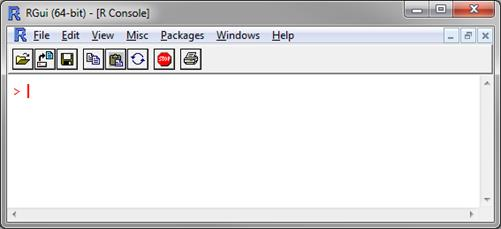 Figure 1. R command window
 -
Change your current working directory to the R directory in the Techila SDK.
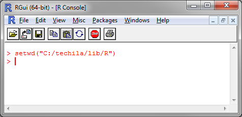 Figure 2. Changing the current working directory.
 -
Install the
techilapackage using the following command:install.packages("techila", type = "source", repos = NULL, INSTALL_opts = "--no-multiarch")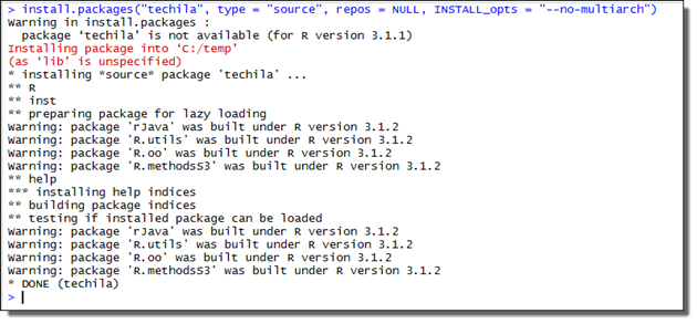 Figure 3. Installing without multiarch.
The
techilapackage is now ready for use. You can verify that the package was installed correctly by loading the package with the following command:library(techila)
Note! Depending on your R-version, certain functions might masked by the functions in the other required packages. If you wish to use a masked function from a specific package, this can be achieved with
<package>::<function>notation.After loading the
techilapackage you can display thepeachandcloudforhelp using commands:?peach ?cloudfor
1.2. Updating the techila Package
This Chapter contains instructions for updating the techila package. These steps will need to be performed when upgrading to a newer Techila SDK version.
-
Detach the old
techilapackage using command:detach("package:techila")If the
techilapackage not loaded when the command above is executed, you might receive a corresponding error message. You can ignore this error message and continue with the update process.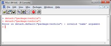 Figure 4. Detaching the package.
 -
Change your current working directory in R to the
<full path>/techila/lib/R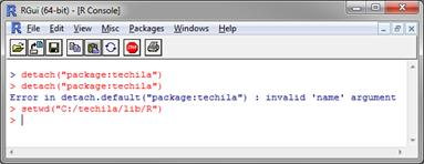 Figure 5. Changing current working directory.
 -
Install the new
techilapackage using command:install.packages("techila", type = "source", repos = NULL, INSTALL_opts = "--no-multiarch")The
techilapackage has now been updated.
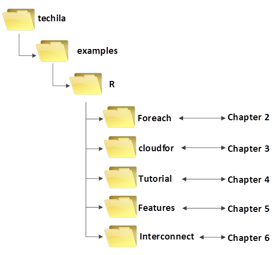
1.3. Example Material
The R scripts containing the example material discussed in this document can be found in the Foreach, Tutorial, Features, cloudfor and Interconnect folders in the Techila SDK. These folders contain subfolders, which further contain the actual R scripts that can be used to run the examples. Foreach Backend Examples contains walkthroughs of code samples that use the TDCE foreach backend. Cloudfor Examples contain examples for the cloudfor function. Peach Tutorial Examples and Peach Feature Examples contain walkthroughs of code samples that use the peach function. Interconnect contains walkthroughs of examples that use the Techila interconnect feature to transfer interconnect data packages between Jobs.
1.4. Naming Convention of the R Scripts
The typical naming convention of R scripts presented in this document is explained below:
-
R scripts ending with
distcontain the Techila Worker Code, which will be distributed to the Techila Workers when the Local Control Code is executed. -
R scripts beginning with
run_contain the Local Control Code, which will create the computational Project when executed locally on the End-User’s own computer. -
R scripts beginning with
local_contain locally executable code, which does not communicate with the TDCE environment.
Please note that some R scripts and functions might be named differently, depending on their role in the computational Project.
1.5. R Foreach Backend
The techila package includes a foreach backend. After registering the backend, operations inside foreach structures can be pushed to the TDCE environment by using the %dopar% notation.
The backend can be registered with the following commands:
library(techila)
registerDoTechila()
After registering the command, operations in foreach structures can be executed by using the %dopar% notation as illustrated in the example code snippet below. When executed, this example code snippet would create a Project consisting of three Jobs. Each Job would calculate the square root of the loop counter value.
library(techila)
library(foreach)
registerDoTechila()

result <- foreach(i=1:3) %dopar%
{
  sqrt(i)
}
When registering the backend with the registerDoTechila function, additional parameters can be used to add or modify functionality.
The default behavior of the Techila foreach backend will execute one iteration in each Job. This means that if you have 1000 iterations, the Project will contain 1000 Jobs. If these iterations are computationally light (in the range of a second or two per iteration), you can improve performance by grouping several iterations into each Job by using the steps parameter. For example, the following syntax could be used to define that 10 iterations would be performed in each Job, reducing the number of Jobs in the Project to 100.
library(techila)
registerDoTechila(steps=10)
result <- foreach(i=1:1000) %dopar%
{
  sqrt(i)
}
In situations where your computations have dependencies to R packages that are not included in the standard R distribution in your computations, you can mark them for transfer by using the packages parameter. The example below could be used to transfer pracma and gbm packages from the End-User’s computer to the Techila Workers.
library(techila)
registerDoTechila(packages=list("pracma","gbm"))
It is also possible to use perfectly nested foreach loop structures. In perfectly nested loop structures, all content is inside the innermost loop as illustrated in the code snippet below.
library(techila)
library(foreach)
registerDoTechila()

foreach(b=1:4, .combine=`cbind`) %:%
    foreach(a=1:3) %dopar% {
      a* b
    }
The foreach backend also enables computations from other functions that use the foreach backend to be executed in TDCE. This includes functionality in e.g. the plyr and the caret packages. The code snippets below illustrate how TDCE can be used with the ddply function from the plyr package (Example 1) and the train function from the caret package (Example 2).
Example 1: plyr ddply
library(techila)
library(plyr)
registerDoTechila()

res <- ddply(iris, .(Species), numcolwise(mean) ,.parallel = TRUE))
Example 2: caret train
# Load the packages needed in the example
library(mlbench)
library(techila)
library(caret)

registerDoTechila(packages=list("gbm","e1071"), # Additional packages needed on Workers..
                  steps=10) # Defines how many loops are done in each Job.

data(Sonar)

inTraining <- createDataPartition(Sonar$Class, p = .75, list = FALSE)
training <- Sonar[ inTraining,]
testing  <- Sonar[-inTraining,]

# 10-fold CV
fitControl <- trainControl(
  method = "repeatedcv",
  number = 10,
  repeats = 10)

# Compute in TDCE
result <- train(Class ~ ., data = training,
                 method = "gbm",
                 trControl = fitControl,
                 verbose = FALSE)
1.6. R Peach Function
The peach function provides a simple interface that can be used to distribute even the most complex programs. When using the peach function, every input argument is a named parameter. Named parameters refer to a computer language’s support for function calls that clearly state the name of each parameter within the function call itself.
A minimalistic R peach syntax typically includes the following parameters:
-
funcname
-
params
-
files
-
peachvector
-
datafiles
Using these parameters, the End-User can define input parameters for the executable function and transfer additional files to the Techila Workers. An example of a peach function syntax using these parameters is shown below:
peach(funcname="name_of_the_function_that_will_be_called",
      params=list(variable_1,variable_2),
      files=list("R_script_that_will_be_sourced.R"),
      datafiles=list("file_1"),
      peachvector=1:jobs)
Tutorial examples on the use of these parameters can be found in Peach Tutorial Examples. General information on available peach parameters can also be displayed by executing the following commands in R.
library(techila)

?peach
1.7. R Cloudfor Function
The cloudfor function provides an even more simplistic way to distribute computationally intensive for-loop structures to the TDCE environment. The cloudfor function is based on the peach function, which means that all peach features are also available in cloudfor.
The loop structure that will be distributed and executed on Techila Workers is marked by replacing the for-loop with a cloudfor-loop. In addition, the syntax for defining the loop iterations is slightly modified as illustrated in the image below.
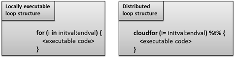
for-loop structures to cloudfor-loop structures enables you to execute the computationally intensive operations in the Techila Distributed Computing Engine environment.The <executable code> notation in the example above represents the algorithm that will be executed during each iteration of the loop structure.
The iteration interval in the cloudfor version is given as a vector ranging from initval to endval. These variables to the same values as in the locally executable for-loop, representing the start and end values for the loop iterations.
The %t% notation in the cloudfor version defines that the following code block enclosed in curly brackets should be executed in the TDCE environment. When using multiple cloudfor-loops, the outer cloudfor-loops are defined with a %to% notation and the %t% notation is used do define the innermost cloudfor-loop. A code sample illustrating multiple nested loops can be found later in this Chapter.
Please note that iterations of the cloudfor-loop might be performed different Techila Workers, meaning all computational operations must also be independent. For example, the conversion shown below is possible, because all the iterations are independent.
| Locally Executable | Distributed Version |
|---|---|
|
|
But it is NOT possible to convert the loop structure shown below. This is because the value of A in the current iteration (e.g. i=3) depends on the value of the previous iteration (i=2).
| Locally Executable | Distributed Version |
|---|---|
|
Conversion NOT Possible. Recursive dependency in the local |
When the cloudfor keyword is encountered, all variables and functions that are required to execute the code on the Techila Worker are automatically transferred and made available on the Techila Worker.
The number of Jobs in the Project will be automatically set by evaluating the execution time of iterations locally. In cases where the execution of a single iteration is short, multiple iterations will be performed in each Job. If the execution time of a single iteration is long (by default more than 20 seconds), one iteration will be performed in each Job. The number of iterations performed in a single Job can also be controlled with the .steps control parameter as shown below.
A <- cloudfor(i=1:10,.steps=2) %t% {
     <executable code>
     }
In the example above, two iterations would be performed in each Job. This would create a Project containing five (5) Jobs, because the maximum value of the loop counter is ten (10).
Because cloudfor is based on peach, you can also use peach parameters by prepending the name of the parameter with a dot (.<peach parameter>).This is illustrated in the syntax below, where the streaming feature has been enabled with the .stream parameter.
A <- cloudfor(i=1:10,.steps=2,
                   .stream=TRUE) %t% {
     <executable code>
     }
It is also possible to distribute perfectly nested loop structures. In perfectly nested for-loops, all content is inside the innermost for-loop. This means that if you have a locally executable perfectly nested for-loop structure, you can distribute the computations to the TDCE environment by marking the executable code as shown below.
A <- cloudfor (i = 1:10) %to%
       cloudfor (j = 1:10) %t% {
        <executable code>
     }
When using multiple, perfectly nested cloudfor-loops, the outer loops are defined with the %to% notation. The innermost cloudfor-loop is defined with the %t% notation, which also indicates that the code in the following curly brackets should be executed in the TDCE environment.
In situations where you have several, perfectly nested cloudfor-loops, only the innermost loop is marked with the %t% notation. All other loops are marked with %to%. This is illustrated below:
A <- cloudfor (i = 1:10) %to%
         cloudfor (j = 1:10) %to%
             cloudfor (k = 1:10) %t% {
    <executable code>
  }
It is also possible to evaluate regular for-loop structures inside cloudfor-loops. For example, the syntax shown below would evaluate the innermost for-loop (j in 1:10) in each Job.
A <- cloudfor (i = 1:10) %t% {
       <executable code 1>
       for (j in 1:10) {
        <executable code 2>
       }
       <executable code 3>
       return(<your result data>) # This will be returned from each Job.
     }
However, it is NOT possible to use cloudfor-loops on the same level when inside a cloudfor-loop.
A <- cloudfor (i = 1:10) %to%
       cloudfor (j = 1:10) %t% {
        <executable code>
     }
     cloudfor (k = 1:10) %t% {
        <more executable code>
     }
General information on available control parameters can also be displayed by executing the following command in R.
library(techila)
?cloudfor
?peach
Please note that cloudfor-loops should only be used to divide the workload in computationally expensive for-loops. If you have a small number of computationally light operations, using a cloudfor-loop will not result in better performance.
As an exception to this rule, some of examples discussed in this document will be relatively simple, as they are only intended to illustrate the mechanics of using the cloudfor function.
1.8. Process Flow
When a Project is created with peach or cloudfor, each Job in a computational Project will have a separate R workspace. Functions and variables are loaded the preliminary stages of each computational Job by sourcing the R-files defined in the files parameter (when using peach) and by loading the parameters stored in the techila_peach_inputdata file.
When a Job is started on a Techila Worker, the peachclient.r script (included in the techila package) is called. The peachclient.r file is an R script that acts as a wrapper for the Techila Worker Code and is responsible for transferring parameters to the executable function and for returning the final computational results. This functionality is hidden from the End-User. The peachclient.r will be used automatically by computational Projects created with peach or cloudfor.
The peachclient.r wrapper also sets a preliminary seed for the random number generator by using the R set.seed() command. Each Job in a computational Project will receive a unique random number seed based on the current system time and the jobidx parameter. The preliminary random number seeding can be overridden by calling the set.seed() function in the Techila Worker Code with an appropriate random seed.
1.8.1. Peach Function
The list below contains some of the R specific activities that are performed automatically when the peach function is used to create a computational Project.
-
The
peachfunction is called locally on the End-Users computer -
R scripts listed in the
filesparameter are transferred to Techila Workers -
Files listed in the
datafilesparameter are transferred to Techila Workers -
The
peachclient.rfile is transferred to Techila Workers -
Input parameters listed in the
paramsparameter are stored in a file calledtechila_peach_inputdata, which is transferred to Techila Workers. -
The files listed in the
filesanddatafilesparameters and the filestechila_peach_inputdataandpeachclient.rare copied to the temporary working directory on the Techila Worker -
The
peachclient.rwrapper is called on the Techila Worker. -
Variables stored in the file
techila_peach_inputdataare loaded to the R Workspace -
Files listed in the
filesparameter are sourced using the Rsourcecommand -
The
<param>notation is replaced with apeachvectorelement -
The peachclient calls the function defined in the
funcnameparameter with the input parameters -
The peachclient saves the result in to a file, which is returned from the Techila Worker to the End-User
-
The
peachfunction reads the output file and stores the result in a list element (If a callback function is used, the result of the callback function is returned). -
The entire list is returned by the
peachfunction.
1.8.2. Cloudfor Function
The list below contains some of the R specific activities that are performed automatically when using the cloudfor function to create a computational Project.
-
The innermost
cloudforloop (defined by %t%) is encountered in the End-Users local R code -
Execution time required for a loop iteration is estimated
-
The code block within the innermost
cloudfor-loop is stored in the filetechila_peach_inputdata. -
Additional functions and workspace variables required when executing the Techila Worker Code are stored in the
techila_peach_inputdatafile, which is transferred to the Techila Workers. -
The
peachclient.randtechila_for.rfiles are transferred to the Techila Workers -
The
peachclient.rwrapper is called on the Techila Worker -
The peachclient loads the variables and functions stored in the
techila_peach_inputdatafile to the workspace -
The peachclient calls the
techila_for.rwrapper for the specified number of iterations -
The
techila_for.rwrapper executes the code block each time it is called -
Results from the loop iterations are saved in list form to an output file, which is returned from the Techila Worker
-
Output files are read on the End-Users computer and results are stored as list elements
-
The entire list is returned as the result
2. Foreach Backend Examples
This Chapter contains examples on how to use the Techila Distributed Computing Engine (TDCE) foreach backend to execute computations in a TDCE environment. The example material discussed in this Chapter, including R scripts and data files can be found in the subdirectories under the following folder in the Techila SDK:
techila\examples\R\Foreach
2.1. Executing Foreach Computations in Techila Distributed Computing Engine
This example shows how to use the foreach backend to execute computations in a TDCE environment by using the foreach %dopar% notation
The material discussed in this example is located in the following folder in the Techila SDK:
techila\examples\R\Foreach\foreach
Note! In order to run this example, the foreach package needs to be installed.
Before you are able to use the TDCE foreach backend, you will need to load the TDCE library and register the backend with the following R commands:
library(techila)
registerDoTechila(sdkroot = "<path to your `techila` directory>")
The notation in <> needs to be replaced with the location of your Techila SDK’s techila directory. For example, if your Techila SDK is located in C:/techila, then you could register the backend with the following syntax.
registerDoTechila(sdkroot = "C:/techila")
After registering the TDCE foreach backend, computational operations in foreach structures can be executed in a TDCE environment by using the %dopar% notation as shown in the example snippet below.
result <- foreach(i=1:5) %dopar%
{
  i*i
}
The example code snippet above would create a Project consisting of five Jobs. Each Job execute one iteration of the foreach loop structure. The result would be stored in the result variable in list format.
In situations where the computational operations performed in a single iteration are computationally light, it would be inefficient to create one Job for each iteration. A more efficient implementation can be done by using the .steps parameter to define a suitably large number of iterations for each Job. This is illustrated in the code snippet below.
result <- foreach(i=1:10000, .options.steps=5000) %dopar%
{
  i*i
}
The example code snippet above consists of 10000 iterations. The example code snippet also defines that 5000 iterations should be executed in each Job. This means that when the example code snippet is executed, it would create a Project consisting of two Jobs, where each Job would compute 5000 iterations.
All parameters available for peach can also be used with foreach. The general syntax for defining parameters is:
.options.<peach parameter>
For more information about available peach parameters, please see:
?peach
The TDCE foreach backend also supports using the foreach .combine option to control how the results are managed.
2.1.1. Foreach example walkthrough
The foreach example included in the Techila SDK is shown below:
# Example documentation: http://www.techilatechnologies.com/help/r_foreach_foreach
# Copyright Techila Technologies Ltd.

# Uncomment to install required packages if required.
# install.packages("iterators")
# install.packages("foreach")

run_foreach <- function() {
  # This function registers the Techila foreach backend and uses the %dopar%
  # notation to execute the computations in parallel, in the Techila
  # environment.
  #
  # Example usage:
  #
  # source('run_foreach.r')
  # res <- run_foreach()

  # Load required packages
  library(techila)
  library(foreach)

  # Register the Techila foreach backend and define the 'techila' folder
  # location.
  registerDoTechila(sdkroot = "../../../..")

  iters=10

  # Create the Project using foreach and %dopar%.
  result <- foreach(i=1:iters,
                    .options.steps=2, # Perform 2 iterations per Job
                    .combine=c # Combine results into numerical vector
                    ) %dopar% { # Execute computations in parallel
       sqrt(i) # During each iteration, calculate the square root value of i
     }

  # Print and return results.
  print(result)
  result
}
This example will create a Project consisting of five Jobs. The code starts by loading the required packages: techila and foreach.
After this, the TDCE foreach backend is registered and the Techila SDK’s techila directory location is defined.
The foreach syntax used to perform the computations in TDCE starts by defining that the computational result should be stored in variable result and that the number of iterations should range from 1 to 10.
Each Job will perform two iterations. Because the total number of iterations was set to 10, this means the Project will consist of five Jobs.
The results will be combined with the c operator. This means that the results will be returned as a numerical vector, instead of a list.
The %dopar% notation will push the computations to the TDCE environment. (If you would change this to %do%, the operations would be executed sequentially on your computer.)
The code that will be executed in each iterations is quite trivial, consisting of simply calculating the square root of the loop counter i.
After the Project has been completed, the results will be returned from the TDCE environment and printed to the R console on your computer.
2.1.2. Creating the Project
To create the computational Project, change your current working directory in your R environment to the directory that contains the example material relevant to this example.
After having browsed to the correct directory, you can source the Local Control Code using command:
source("run_foreach.r")
After having sourced the file, create the computational Project using command:
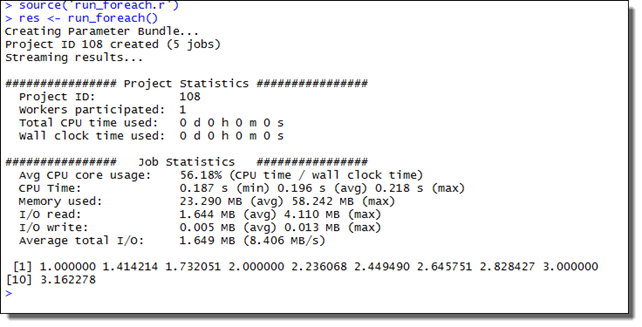
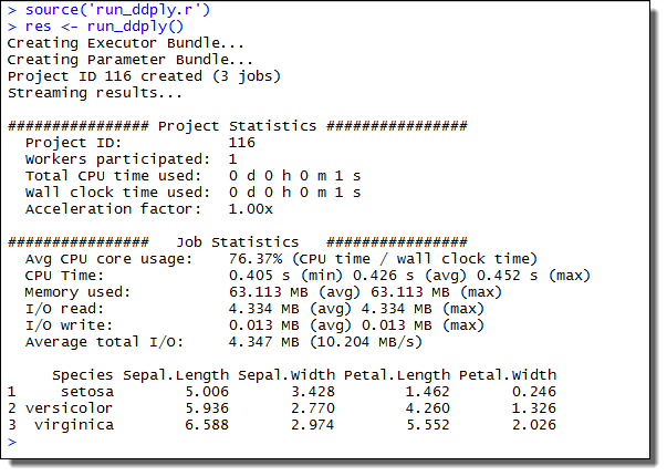
res <- run_foreach()
This will create a Project consisting of five Jobs, each Job performing two iterations of the foreach loop structure. The example screenshot below illustrates what the expected output looks like.
2.2. Using the Techila Distributed Computing Engine Foreach Backend with Plyr Functions
The material discussed in this example is located in the following folder in the Techila SDK:
techila\examples\R\Foreach\plyr
Note! In order to run this example, the foreach and plyr packages needs to be installed.
When using functions from the plyr package to perform computations, the .parallel option can be used to perform computations in parallel, using the backend provided by foreach. This means that after registering the TDCE foreach backend, computations can be executed in TDCE with the .parallel option.
Note! In order to the TDCE backend with functions in the plyr package, the plyr package will need to be transferred to the Techila Workers using the .packages parameter. The plyr package contains platform specific files (.dll for Windows and .so for Linux), meaning the Techila Workers must have the same operating system as the one you are using on your R workstation. In other words, if you are using a Windows computer, the Techila Workers must also have a Windows operating system.
2.2.1. Executing plyr functions in parallel
In order to execute function from the plyr package in parallel using TDCE, the following packages need to be loaded: techila and plyr. After loading the packages, the TDCE backend can be registered using the syntax illustrated below
library(techila)
library(plyr)
registerDoTechila(sdkroot = "<path to your `techila` directory>")
The notation in <> needs to be replaced with the location of your techila directory. For example, if your Techila SDK is located in C:/techila, then you could register the backend with the following syntax.
registerDoTechila(sdkroot = "C:/techila")
After registering the TDCE backend, functions from the plyr package can be executed in a TDCE environment by setting .parallel=TRUE as shown in the example snippet below.
res <- aaply(ozone,
             1,
             mean,
             .parallel=TRUE,
             .paropts=list(.options.packages=list("plyr")))
The array ozone is included in the plyr package and is a 24 x 24 x 72 numeric array. The code snippet above would calculate the average value for each row in the ozone array in a separate Job, meaning the Project would consist of 24 Jobs. The plyr package has been transferred to the Techila Workers by using the .packages parameter.
2.2.2. Example walkthrough
This example illustrates how the computations performed with ddply can be executed in parallel in a TDCE environment. The example uses the iris data frame, which is included in the plyr package. The code for the example in the Techila SDK is shown below:
# Example documentation: http://www.techilatechnologies.com/help/r_foreach_plyr
# Copyright Techila Technologies Ltd.
#
# Uncomment to install required packages if required.
# install.packages("plyr")
# install.packages("iterators")
# install.packages("foreach")

run_ddply<- function() {
  # This function registers the Techila foreach backend and uses the
  # .parallel option in ddply to execute computations in parallel,
  # in the Techila environment.
  #
  # Example usage:
  #
  # source('run_ddply.r')
  # res <- run_ddply()

  # Load required packages.
  library(techila)
  library(plyr)

  # Register the Techila foreach backend and define the 'techila' folder
  # location.
  registerDoTechila(sdkroot = "../../../..")

  # Create the computational Project using ddply with the .parallel=TRUE option.
  result <- ddply(iris,         # Split this data frame
                  .(Species),   # According to the values in the Species column
                  numcolwise(mean), # And perform this operation on the column data.
                  .parallel=TRUE # Process the computations in Techila
                  )

  # Print and return results
  print(result)
  result
}
The code starts by loading the required packages: techila and plyr. After loading the packages, the TDCE foreach backend is registered and the Techila SDK’s techila directory location is defined.
The operation will be performed on data frame iris, which will be split into parts according values in Species . The operation numcolwise(mean) will be executed for each data frame part. The computations are marked for parallel execution and the required plyr package will be transferred to all participating Techila Workers.
The iris data frame contains three unique values in the Species column and the data for each Species will be processed in a single Job. This means that the Project will consist of three Jobs.
2.2.3. Creating the Project
To create the computational Project, change your current working directory in your R environment to the directory that contains the example material relevant to this example.
After having browsed to the correct directory, you can source the Local Control Code using command:
source("run_ddply.r")
After having sourced the file, create the computational Project using command:
res <- run_ddply()
This will create a Project consisting of three Jobs, each Job processing the data for one Species. The example screenshot below illustrates what the expected output looks like.
3. Cloudfor Examples
This Chapter contains walkthroughs of the example material that uses the cloudfor function included in the Techila SDK. The examples in this Chapter highlight the following subjects:
-
Controlling the Number of Iterations Performed in Each Job
-
Transferring Data Files
-
Managing Streamed Results
The example material used this Chapter, including R-scripts and data files can be found in the subfolders under the following folder in the Techila SDK:
techila\examples\R\cloudfor\<example specific subfolder>
Please note that the example material in this Chapter is only intended to highlight some of the available features in cloudfor. For a complete list of available control parameters, execute the following command in R.
library(techila)

?cloudfor
3.1. Controlling the Number of Iterations Performed in Each Job
This example is intended to illustrate how to convert a simple, locally executable for-loop structure to a cloudfor-loop structure. Executable code snippets are provided of a locally executable loop structure and the equivalent cloudfor implementation. This example also illustrates on how to control the number of iterations performed during a single Job.
The material used in this example is located in the following folder in the Techila SDK:
techila\examples\R\cloudfor\1_number_of_jobs
When using cloudfor to distribute a loop structure, the maximum number of Jobs in the Project will be automatically limited by the number of iterations in the loop structure. For example, the loop structure below contains 10 iterations, meaning that the maximum number of Jobs in the Project would be 10.
cloudfor(counter=1:10) %t% {
  <executable code>
}
By default, cloudfor will estimate the execution time of iterations locally on the End-Users computer. This is done by executing the code block (as represented by the <executable code> notation) for a minimum of one second. Based on the number of iterations performed during this estimation, each Job will be assigned a suitable number of loop iterations so that each Job will last for a minimum of 20 seconds.
If no iterations have been completed within one second, the evaluation will continue for a maximum of 20 seconds. If no iterations have been completed after evaluating the code block for 20 seconds, the number of iterations in each Job will be set to one (1).
If you require more control over the number of iterations that will be performed in each Job, this can be achieved by using the .steps control parameter. The general syntax for using this control parameter is shown below:
cloudfor(counter=1:10,.steps=<iterations>) %t% {
  <executable code>
}
The <iterations> notation can be used to define the number of iterations that should be performed in each Job. For example, the syntax shown below would define that each two iterations should be performed in each Job.
cloudfor(counter=1:10,.steps=2) %t% {
  <executable code>
}
Please note that when using the .steps parameter, you will also fundamentally be defining the length of a single Job. If you only perform a small number of short iterations in each Job, the Jobs might be extremely short, resulting poor overall efficiency. It is strongly advised to use values that ensure the execution time of a Job will not be too short.
3.1.1. Locally executable program
The locally executable program used in this example is shown below.
# Example documentation: http://www.techilatechnologies.com/help/r_cloudfor_1_number_of_jobs
# Copyright Techila Technologies Ltd.
local_function <- function(loops) {
# This function will be executed locally on your computer and will not
# communicate with the Techila environment.
#
# Example usage:
#
# loops <- 100
# result <- local_function(loops)
result <- rep(0, loops) # Create empty array for results
for (i in 1:loops) {
result[i] = i * i # Store result in array
}
result
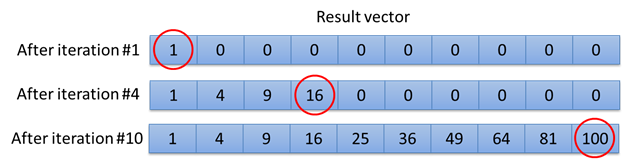
}The code contains a single for-loop, which contains a single multiplication operation where the value of the i variable is squared. The value of the i variable will be replaced with the iteration number, which will be different each iteration. The result of the multiplication will be stored in the result vector at the index determined by the value of the i variable.
The locally executable program can be executed by changing your current working directory in R to the directory containing the material for this example and executing the command shown below:
source("local_function.r")
result <- local_function(10)
Executing the command shown above will calculate 10 iterations. The values stored in the result-array are shown in the image below.
i.3.1.2. The cloudfor version
The cloudfor version of the locally executable program is shown below.
# Example documentation: http://www.techilatechnologies.com/help/r_cloudfor_1_number_of_jobs
# Copyright Techila Technologies Ltd.

library(techila)

run_jobs <- function(loops) {
  # This function contains  the distributed version, where operations inside the
  # loop structure will be executed on Workers.
  #
  # Example usage:
  #
  # loops <- 100
  # result <- run_jobs(loops)

  result <- cloudfor (i=1:loops,
                      .sdkroot="../../../..", # Path of the techila folder
                      .steps=2 # Perform two iterations per Job
                     ) %t% {  # Start of code block that will be executed on Workers
      i * i # This operation will be performed on the Workers
  } # End of code block executed on Workers
}
The command library(techila) will be executed when the file is sourced. After executing the command, the functions in the techila-package will be available.
The for-loop in the locally executable version has been replaced with a cloudfor-loop. The %t% notation after the cloudfor-loop defines that the code inside the following curly brackets should be executed in the Techila Distributed Computing Engine (TDCE) environment. In this example, the executable code block only contains the operation where the value of the i variable is squared.
The .sdkroot control parameter is used to define the location of the techila directory. In this example, a relative path definition has been used. This definition will be used in all of the R example material in the Techila SDK.
The .steps control parameter is used to define that two iterations should be calculated in in each Job. This means that for example if the number of loops is set to 10, the number of Jobs will be 5 (number of loops divided by the value of the steps parameter).
3.1.3. Creating the computational project
The computational Project can be created by executing the cloudfor version of the program. The cloudfor version can be executed by changing your current working directory in R to the directory containing the material for this example and executing the command shown below:
source("run_jobs.r")
result<-run_jobs(10)
After you have executed the command, the Project will be automatically created and will consist of five (5) Jobs. These Jobs will be assigned and computed on Techila Workers in the TDCE environment. Each Job will compute two iterations of the loop structure and will return a list containing two values returned from the loop evaluations. This list will be stored in an output file, which will be automatically transferred to the Techila Server.
After all computational Jobs have been completed the result files will be transferred to your computer from the Techila Server. The values stored in the output files will be read and stored in the result-array. This array will contain all the values from the iterations and will correspond to the output generated by the locally executable program discussed earlier in this Chapter.
3.2. Transferring Data Files
This example illustrates how to transfer data files to the Techila Workers. This example uses two different data file transfer methods:
-
Transferring common data files required on all Techila Workers
-
Transferring Job-specific data files
The material used in this example is located in the following folder in the Techila SDK:
techila\examples\R\cloudfor\2_transferring_data_files
Data files that are required on all Techila Workers can be transferred to Techila Workers with the .datafiles control parameter. All transferred data files will be copied to the same temporary working directory with the Techila Worker Code.
For example, the following syntax would transfer a file called file1 to all participating Techila Workers.
.datafiles=list("file1")
Several files can be transferred by entering the names of the files as a comma separated list. For example, the following syntax would transfer files called file1 and file2 to all participating Techila Workers
.datafiles=list("file1","file2")
The syntaxes shown above assume that the files are located in the current working directory. To specify a different location for a file, prepend the file name with the path of the file. For example, the syntax shown below would retrieve file1 from the current working directory and file2 from the directory C:/temp.
.datafiles=list("file1","C:/temp/file2")
Job-specific input files can be used in situations where only some files of a data set are required during any given Job. The Job-specific input files feature can be used with the .jobinputfiles control parameter. The general syntax for defining the control parameter is shown below.
.jobinputfiles=list(
   datafiles = list(<comma separated list of file names>),
   filenames = list(<name(s) of the Job-specific input file(s) on the Worker>)
 )
Note! When using Job-specific input files, the number of files listed in the datafiles parameter must be equal to the number of Jobs in the Project. This means that the use of the .steps control parameter is typically required for ensuring that the Project contains a correct number of Jobs.
An example syntax is shown below.
 result <- cloudfor(i=1:2,
                   .steps=1,
                   .jobinputfiles=list(
                       datafiles = list("file1","file2"),
                       filenames = list("input.data"))) %t% {
                   <executable code>
}
In the example above, the value of the .steps parameter is set to one (1), which means that one (1) iteration will be performed in each Job. As the total number of iterations in the loop structure is two (2), this ensures that the Project will contain two (2) Jobs. Setting the number of Jobs to two (2) is required because the number of Job-specific input files is also two (2). File file1 will be transferred to Job 1 and file file2 will be transferred to Job 2. After the files have been transferred to the Techila Workers, each file will be renamed to input.data.
Information on how to define multiple Job-specific input files can be found in Job Input Files.
3.2.1. Locally executable program
The locally executable program used in this example is shown below.
# Example documentation: http://www.techilatechnologies.com/help/r_cloudfor_2_transferring_data_files
# Copyright Techila Technologies Ltd.

local_function <- function() {
  # This function will be executed locally on your computer and will not
  # communicate with the Techila environment.
  #
  # Usage:
  #
  # result <- local_function()

  # Read values from the data files
  values <- read.table("datafile.txt", header=TRUE, as.is=TRUE)
  targetvalue <- read.table("datafile2.txt", header=TRUE, as.is=TRUE)

  # Determine the number of rows and columns of data
  rows <- nrow(values)
  cols <- ncol(values)

  # Create empty matrix for results
  result <- matrix(rep(NA, 12), rows, cols)

  for (i in 1:rows) { # For each row of data

    data <- values[i,] # Read the values on the row
    for (j in 1:cols) { # For each element on the row

      # Compare values on the row to the ones on the target row
      if(identical(values[[i, j]], targetvalue[[j]])) {
        result[i, j] <- TRUE  # If rows match
      }
      else {
        result[i, j] <- FALSE # If rows don't match
      }
    }
  }
  print(result)
  result
}
During the initial steps of the program, the tables stored in files datafile.txt and datafile2.txt will be read and stored the variables values and targetvalue respectively. The targetvalue variable will contain one row of data and the values variable will contain four rows of data with a similar structure.
The computational part consists of comparing the values of the rows stored in the values variable with the row stored in the targetvalue variable. Each line is compared during a separate iteration of the outermost for-loop. A graphical illustration of the data is shown in the image below.
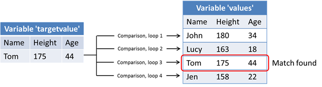
for-loop iterations. A matching row will be found during the 3rd iteration.The result of the comparison will be stored in the result-matrix, which will contain a row of FALSE values for rows that did not match. The matching row will be marked with TRUE values.
The locally executable program can be executed by changing your current working directory in R to the directory containing the material for this example and executing the command shown below:
source("local_function.r")
result <- local_function()
3.2.2. The cloudfor version
The cloudfor version of the locally executable program is shown below. Line numbers have been added.
# Example documentation: http://www.techilatechnologies.com/help/r_cloudfor_2_transferring_data_files
# Copyright Techila Technologies Ltd.

library(techila)

run_datafiles <- function() {
  # This function contains  the distributed version, where operations inside the
  # loop structure will be executed on Workers.
  #
  # Usage:
  #
  # result <- run_datafiles()


  # Read values from the data file
  values <- read.table("datafile.txt", header=TRUE, as.is=TRUE)

  # Determine the number of rows and columns of data
  rows <- nrow(values)
  cols <- ncol(values)

  # Create empty matrix for results that will be generated in one Job
  result <- matrix(rep(NA, 3), 1, 3)

  # Split the data read from file 'datafile.txt' to multiple files.
  # These files will be stored i the Job Input Bundle.
  for (i in 1:rows) {
    data <- values[i,]
    write.table(data, file=paste("input", as.character(i), sep=""))
  }

  # Create a list of the files generated earlier.
  inputlist <- as.list(dir(pattern="^input_*"))

  result <- cloudfor(i=1:rows,
                    .steps=1, # One iteration per Job
                    .sdkroot="../../../..", # Path to the 'techila' folder
                    .datafiles=list("datafile2.txt"), # Common data file for all Jobs
                    .jobinputfiles=list(              # Create a Job Input Bundle
                       datafiles = inputlist,         # List of files that will be placed in the Bundle
                       filenames = list("input"))     # Name of the file on the Worker
                     ) %t% { # Start of the code block that will be executed on Workers

    targetvalue <- read.table("datafile2.txt", header=TRUE, as.is=TRUE)
    values <- read.table("input", header=TRUE, as.is=TRUE)

    # Compare the values stored in the common data file ('datafile2.txt') with
    # the ones stored in teh Job-specific input file.
    for (j in 1:cols) { # For each element
        if(identical(values[[j]], targetvalue[[j]])) { # Compare element
          result[1, j] <- TRUE  # If elements match
        }
        else {
          result[1, j] <- FALSE # If elements do not match
        }
      }

    result # Return the 'result' variable

    } # End of the code block executed on Workers

  # Make result formatting match the one in the local version
  result <- matrix(unlist(result), rows, cols, byrow=TRUE)

  # Display result
  print(result)
  result
}
The code starts by loading the techila package, making the functions in the package available.
After loading the package, the code will load the table in file datafile1.txt, store the values to the values variable and determine the number of columns and rows in the table. An empty result array will also be created, which will be used to store row comparison results on the Techila Worker.
Before creating a Project, the code will execute an additional local for-loop. This loop will be used to create four (4) new files. Each file will contain one row of data extracted from the file datafile1.txt.The first row will be stored in a file called input_1, the second row in a file called input_2 and so on. These files will be used as Job-specific input files and will be transferred to the TDCE environment later in the program.
After generating the files, a list containing all file names starting with input that are located in the current working directory will be created. This list will be used later in the program to define a list of files that should be used as Job-specific input files.
The cloudfor-loop used in this example will range from one (1) to number of rows in the entire data table. The results of the computational Project will be stored in the result variable.
The number of iterations performed in each Job will be set to one (1) by using the .steps parameter. This means that the Project will contain four (4) Jobs, one Job for each row of data.
The location of the techila directory is set with the .sdkroot parameter.
The .datafiles parameter defines that datafile2.txt should be transferred to all participating Techila Workers.
Respectively, the .jobinputfiles parameter is used to transfer Job specific input files. In this example, the filenames parameter contains one list item, meaning one file will be given for each Job. File input1 will be assigned for Job 1, file input2 for Job 2 and so on. Each file will be renamed to input after it has been transferred to the Techila Worker.
After transferring these files to the Worker(s), they will be loaded using the following two lines:
targetvalue <- read.table("datafile2.txt", header=TRUE, as.is=TRUE)
values <- read.table("input", header=TRUE, as.is=TRUE)
These lines will be read the contents of datafile2.txt (will be same in each Job) and input (will be different in each Job).
After reading the files, a similar element-wise comparison will be performed as in the locally executable program. The result of the comparison will be stored in variable result and returned from the Job.
After the Project has been completed, the cloudfor function will return and the results will be stored in variable result.
Creating the computational project
The computational Project can be created by executing the cloudfor version of the program. To execute the program change your current working directory in R to the directory containing the material for this example and execute the command shown below:
source("run_datafiles.r")
result<-run_datafiles()
The Project will contain four (4) Jobs. Each Job will compare the row stored in the Job-specific input file with the row in the file datafile2.txt. The result of the comparison will be stored in the result-array, which will be returned from the Techila Worker.
After all Jobs have been completed, the results will be transferred to the End-Users computer. The results returned by the cloudfor-loop will be in a list form. The values in the list will the stored in a matrix, which will be identical as in the locally executable version.
3.3. Managing Streamed Results
This example illustrates how to use the Streaming and Callback function features with the cloudfor function.
The material used in this example is located in the following folder in the Techila SDK:
techila\examples\R\cloudfor\3_streaming_callback
Streaming can be enabled with the .stream control parameter using the syntax shown below:
.stream=TRUE
When Streaming is enabled, Job results will be transferred from the Techila Server as soon as they are available. The results returned from the Techila Server will be stored at the correct indices by using an index value which will be automatically included with each returned result file.
Callback functions can be enabled with the .callback control parameter using the syntax shown below:
.callback="<callback function name>"
The notation <callback function name> would be replaced with the name of the function you wish to use. For example, the following syntax would call a function called cbFun for each Job result.
.callback="cbFun"
The callback function will receive one (1) input argument, which will contain the value returned from the Techila Worker Code.
Please note that the callback function will be called immediately each time after a new Job result has been received. This means when using Streaming, the call order is not the same as when running a similar loop structure locally. The results returned from the callback function will be placed at the correct indices by cloudfor function.
3.3.1. Locally executable program
The source code of the locally executable program (located in the file local_function.r) used in this example is shown below.
# Example documentation: http://www.techilatechnologies.com/help/r_cloudfor_3_streaming_callback
# Copyright Techila Technologies Ltd.

multiply <- function(a,b){
  # Function containing simple arithmetic operation.
  a * 10 + b
}

local_function <- function() {
  # This function will be executed locally on your computer and will not
  # communicate with the Techila environment.
  #
  # Usage:
  #
  # result <- local_function()

  # Create empty matrix for results
  result <- matrix(0, 2, 3)
  print("Results generated during loop evaluations:")


  for (i in 1:3) {
    for (j in 1:2) {
     # Pass the values of the loop counters to the 'multiply' function and
      # store result in the 'result' matrix
      result[j, i] <- multiply(j, i)
      print(result[j, i]) # Display value returned by the 'multiply' function
    }
  }
  print("Content of the 'result' matrix:")
  print(result)
  result
}
The function called local_function contains two perfectly nested for for-loops. The innermost for-loop will call the multiply function, which will perform some simple arithmetic operations using the loop counter values i and j as input arguments. The result of the operation will be stored in the result-matrix at the indices corresponding to the values of the loop counters i and j. The value of the operation will also be printed each iteration. The content and values stored in the result-matrix are illustrated in the image below.
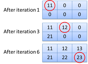
i and j. The value generated during the first iteration (loop counters: i=1,j=1) will be stored at indices (1,1). The value generated during iteration 3 will be stored at indices i=2, j=1 and the last value at indices i=3, j=2.3.3.2. The cloudfor version
The cloudfor version of the locally executable program is shown below.
# Example documentation: http://www.techilatechnologies.com/help/r_cloudfor_3_streaming_callback
# Copyright Techila Technologies Ltd.

library(techila)

cbfun <- function(job_result) {
  # Callback function. Will be called once for each result streamed from the
  # Techila Server.
  print(paste("Job result: ", job_result)) # Display the result
  job_result # Return the result
}

multiply <- function(a, b){
  # Function containing simple arithmetic operation.  Will be automatically
  # made available on the Workers
  a * 10 + b
}

run_streaming <- function() {
  # Function for creating the computational Project.
  project_result <- cloudfor (i = 1:3) %to% # Outer cloudfor loop
                    cloudfor (j = 1:2,
                              .steps=1, # One iteration per Job
                              .callback="cbfun",  # Pass each returned result to function 'cbfun'
                              .stream=TRUE, # Enable streaming
                              .sdkroot="../../../.." # Path to the 'techila' directory
                             ) %t% { # Start of code block that will be executed on Workers
    multiply(j, i) # This operation will be performed on Workers
  } # End of code block executed on Workers

  # After Project has been completed, display results
  print("Content of the reshaped 'result' matrix:")
  print(project_result)
  project_result
}
The cloudfor version contains three functions:
-
run_streaming
-
cbfun
-
multiply
The run_streaming function contains the cloudfor-loops, which have been used to replace the normal for-loops in the locally executable program. In addition, control parameters have been used to enable the result streaming and for defining the name of the callback function.
.stream=TRUE
The parameter shown above will enable individual Job results to be streamed from the Techila Server as soon as they are available. When streaming has been enabled, individual Job results will be returned from the Techila Server in the order the Jobs are completed. This means that the results will be returned in no specific order. The effect of this is illustrated by the callback function, which will display the results in the order in which they will be received from the Techila Server.
.callback="cbfun"
The parameter above defines the function cbfun as the callback function, meaning this function will be used to process each of streamed Job results. In this example, the function will only print the content of the job_result variable, which will contain the value returned from each Job. The values printed during the callback function will most likely be in a different order than in the locally executable version. These results will be automatically reshaped to a 2x3 matrix (same as in the locally executable version) after all results have been received from the Techila Server.
The multiply function is identical as in the locally executable version and contains simple arithmetic operations that use the values of the loop counters as input arguments. This function call is inside the innermost cloudfor-loop, meaning the function will be executed on the Techila Workers.
3.3.3. Creating the computational project
The computational Project can be created by executing the cloudfor version of the program. To execute the program, change your current working directory in R to the directory containing the material for this example and execute the command shown below:
source("run_streaming.r")
result <- run_streaming()
The Project will contain six (6) Jobs. In each of the computational Jobs, the multiply function will be called with different input arguments. The combinations of the input arguments will be identical as in the locally executable program, meaning the operations performed in the computational Jobs will correspond to the operations performed in the locally executable program.
Individual Job results will be streamed in the order they are completed and will be automatically processed by the callback function. After all results have been completed, the results will be reshaped and the matrix containing the results will be printed.
3.4. Active Directory Impersonation
The walkthrough in this Chapter is intended to provide an introduction on how to use Active Directory (AD) impersonation. Using AD impersonation will allow you to execute code on the Techila Workers so that the entire code is executed using your own AD user account.
The material discussed in this example is located in the following folder in the Techila SDK:
techila\examples\R\cloudfor\ad_impersonate
Note! Using AD impersonation requires that the Techila Workers are configured to use an AD account and that the AD account has been configured correctly. These configurations can only be done by persons with administrative permissions to the computing environment.
More general information about this feature can be found in Introduction to Techila Distributed Computing Enginedocument.
Please consult your local Techila Administrator for information about whether or not AD impersonation can be used in your TDCE environment.
AD impersonation is enabled by setting the following Project parameter:
.ProjectParameters = list("techila_ad_impersonate" = "true")
This control parameter will add the techila_ad_impersonate Project parameter to the Project.
When AD impersonation is enabled, the entire computational process will be executed under the user’s own AD account.
3.4.1. Example material walkthrough
The source code of the example discussed here can be found in the following file in the Techila SDK:
techila\examples\R\Features\cloudfor\run_impersonate.r
The code used in this example is also illustrated below for convenience.
# Example documentation: http://www.techilatechnologies.com/help/r_cloudfor_ad_impersonate
run_impersonate <- function() {
# This function contains the cloudfor-loop, which will be used to distribute
# computations to the Techila environment.
#
# During the computational Project, Active Directory impersonation will be
# used to run the Job under the End-User's own AD user account.
#
# Syntax:
#
# source("run_impersonate.r")
# res <- run_impersonate()

# Copyright Techila Technologies Ltd.

  # Load the techila package
  library(techila)

  # Check which user account is used locally
  local_username <- system("whoami",intern=TRUE)

  worker_username <-  cloudfor (i=1:1, # Set the maximum number of iterations to one
                                .sdkroot="../../../..", # Location of the Techila SDK 'techila' directory
                                .ProjectParameters = list("techila_ad_impersonate" = "true") # Enable AD impersonation
  ) %t% {
    # Check which user account is used to run the computational Job.
    worker_username <- system("whoami",intern=TRUE)
  }

  # Print and return the results
  cat("Username on local computer:",local_username, "\n")
  cat("Username on Worker computer:",worker_username, "\n")
  list(local_username,worker_username)
}
The code starts by executing the operating system command whoami, which displays the current domain and user name. This command will be executed on the End-User’s computer, meaning the command will return the End-User’s own AD user name. The user name will be stored in the local_username variable.
The cloudfor-loop used in this example will create a computational Project, which will consist of one Job.
AD impersonation is enabled by using the Project parameter techila_ad_impersonate. With this parameter enabled, the entire computational process will be executed using the End-User’s own AD user account.
The whoami command is then used to get the identity of the Job’s owner on the Techila Worker. Because AD impersonation has been enabled, this command should return the End-User’s AD user name and domain. If AD impersonation would be disabled (e.g. by removing the techila_ad_impersonate Project parameter), this command would return the Techila Worker’s AD user name.
After the Project has been completed, information about which AD user account was used locally and during the computational Job will be displayed.
3.4.2. Creating the Project
To create the computational Project, change your current working directory in your R environment to the directory that contains the example material relevant to this example.
After having browsed to the correct directory, you can source the Local Control Code using command:
source("run_impersonate.r")
After having sourced the file, create the computational Project using command:
res <- run_impersonate()
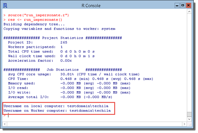
After the Project has been completed, information about the AD user accounts will be displayed. Please note that the output generated by the program will change based your domain and AD account user names. The example screenshot below illustrates the program output when the End-User’s own AD account name is techila and the domain name is testdomain.
3.5. Using Semaphores
The walkthrough in this Chapter is intended to provide an introduction on how to create Project-specific semaphores, which can be used to limit the number of simultaneous operations.
The material discussed in this example is located in the following folder in the Techila SDK:
techila\examples\R\cloudfor\semaphores
More general information about this feature can be found in "Introduction to Techila Distributed Computing Engine" document.
Semaphores can be used to limit the number of simultaneous operations performed in a Project. There are two different types of semaphores:
-
Project-specific semaphores
-
Global semaphores
Project-specific semaphores will need to be created in the code that is executed on the End-User’s computer. Respectively, in order to limit the number of simultaneous processes, the semaphore tokens will need to be reserved in the code executed on the Techila Workers. Global semaphores can only be created by Techila Administrators.
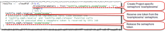
The example figure below illustrates how to use Project-specific semaphores. The semaphore is created by using a Project parameter with a techila_semaphore_ prefix followed by the name of the semaphore. The parameter used in the example will create a Project-specific semaphore called examplesema and with two semaphore tokens.
The functions used for reserving and releasing the semaphore tokens are intended to be executed on the Techila Worker. If these functions are executed on the End-User’s computer, they will generate an error, because these functions are not defined and the End-User’s computer does not have all the necessary TDCE components. For this reason, the .steps control parameter must be used to prevent the code from being executed locally on the End-User’s computer.
The semaphore token will be reserved by the techila.smph.reserve("examplesema") function call. This function call will return when the semaphore token has been reserved from the Project-specific semaphore called examplesema. If no tokens are available, the function will wait until a token becomes available.
The semaphore token will be released by the techila.smph.release("examplesema")function call.
Creating semaphores
As illustrated in the figure above, Project-specific semaphores are created by adding a Project parameter. The following syntaxes can be used when defining the Project parameter:
list("techila_semaphore_<name>" = "size")
list("techila_semaphore_<name>" = "size,expiration")
The list("techila_semaphore_<name>" = "size") syntax creates a Project-specific semaphore with the defined <name> and sets the maximum number of tokens to match the value defined in size. The semaphore tokens will not have an expiration time, meaning the tokens can be reserved indefinitely.
For example, the following syntax could be used to create a semaphore with the name examplesema, which would have 10 tokens. This means that a maximum of 10 tokens can be reserved at any given time.
.ProjectParameters = list("techila_semaphore_examplesema" = "10")
The list("techila_semaphore_<name>" = "size,expiration") syntax defines the <name> and size of the semaphore similarly as the earlier syntax shown above. In addition, this syntax can be used to define an expiration time for the token by using the expiration argument. If a Job reserves a semaphore token for a longer time period (in seconds) than the one defined in the expiration argument, the Project-specific semaphore token will be automatically released and made available for other Jobs in the Project. The process that exceeded the expiration time will be allowed to continue normally.
For example, the following syntax could be used to define a 15 minute (900 second) expiration time for each reserved token.
.ProjectParameters = list("techila_semaphore_examplesema" = "10,900")
Reserving semaphores
As illustrated earlier in the image above, semaphore tokens are reserved by using the techila.smph.reserve function:
techila.smph.reserve(name, isglobal = FALSE, timeout = -1, ignoreerror = FALSE)
When a semaphore token is successfully reserved, the techila.smph.reserve function will, by default, return the value TRUE. Respectively, if there was a problem in the semaphore token reservation process, this function will, by default, generate an error. This behaviour can be modified with the ignoreerror argument as explained later in this Chapter.
The only mandatory argument is the name argument, which is used to define which semaphore should be used. The remaining arguments isglobal, timeout and ignoreerror are optional and can be used to modify the behaviour of the semaphore reservation process. The usage of these arguments is illustrated with example syntaxes below.
techila.smph.reserve(name) will reserve one token from the semaphore, which has the same name as defined with the name input argument. This syntax can only be used to reserve tokens from Project-specific semaphores.
For example, the following syntax could be used to reserve one token from a semaphore named examplesema for the duration of the with-block.
techila.smph.reserve("examplesema")
techila.smph.reserve(name, isglobal=TRUE) an be used to reserve one token from a global semaphore with a matching name as the one defined with the name argument. When isglobal is set to TRUE, it defines that the semaphore is global. Respectively, when the value is set to FALSE, it defines that the semaphore is Project-specific.
For example, the following syntax could be used to reserve one token from a global semaphore called globalsema.
techila.smph.reserve("globalsema", isglobal=TRUE)
techila.smph.reserve(name, timeout=10) can be used to reserve a token from a Project-specific semaphore (or a global semaphore if the syntax defines isglobal=TRUE), which has the same name as defined with the name input argument. In addition, this syntax defines a value for the timeout argument, which is used to define a timeout period (in seconds) for the reservation process. When a timeout period is defined, a timer is started when the constructor requests a semaphore token. If no semaphore token can be reserved within the specified time window, the Job will be terminated and the Job will generate an error. If needed, setting the value of the timeout parameter to -1 can be used to disable the effect of the timeout argument.
For example, the following syntax could be used to reserve one token from Project-specific semaphore called projectsema. The syntax also defines a 10 second timeout value for token. This means that the command will wait for a maximum of 10 seconds for a semaphore token to become available. If no token is available after 10 seconds, the code will generate an error, which will cause the Job to be terminated.
techila.smph.reserve("examplesema", timeout=10)
techila.smph.reserve("examplesema", isglobal=TRUE, timeout=10, ignoreError=TRUE) can be used to define the name, isglobal and timeout arguments in a similar manner as explained earlier. In addition, the ignoreerror argument is used to define that problems during the semaphore token reservation process should be ignore.
If the ignoreerror argument is set to TRUE and there is a problem with the semaphore reservation process, the techila.smph.reserve function will return the value FALSE (instead of generating an error) and the code is allowed to continue normally. If needed, setting ignoreerror to FALSE can be used to disable the effect of this parameter.
The example code snippet below illustrates how to reserve a global semaphore token called globalsema. If the semaphore is reserved successfully, the operations inside the if(reservedok) statement are processed. If no semaphore token could be reserved, code inside the if(!reservedok) statement will be processed.
reservedok=techila.smph.reserve("globalsema",isglobal=TRUE,ignoreerror=TRUE)
if (reservedok)  {
   Execute this code block if the semaphore token was reserved
   successfully.
  techila.smph.release("globalsema",isglobal=TRUE)
}
else if (!reservedok) {
   Execute this code block if there was a problem with the
   reservation process.
}
Releasing semaphores
As mentioned earlier and illustrated by the above code sample, each semaphore token that was reserved with a techila.smph.reserve function call must be released by using the techila.smph.release function:
techila.smph.release(name, isglobal = FALSE)
The effect of the input arguments is explained below using example syntaxes:
The techila.smph.release(name) syntax can be used to release a semaphore token belonging to a Project-specific semaphore with name specified in name. This function cannot be used to release a token belonging to a global semaphore. The example syntax shown below could be used to release a token belonging to a Project-specific semaphore called examplesema.
techila.smph.release("examplesema")
If you want to release a semaphore token belonging to a global semaphore, this can be done by setting the value of the isglobal argument to TRUE.
For example, the following syntax could be used to release a token belonging to a global semaphore called globalsema.
techila.smph.release("globalsema", isglobal=TRUE )
3.5.1. Example material walkthrough
The source code of the example discussed here can be found in the following file in the Techila SDK:
techila\examples\R\Features\cloudfor\run_semaphore.r
The code used in this example is also illustrated below for convenience.
# Example documentation: http://www.techilatechnologies.com/help/r_cloudfor_semaphores
run_semaphore <- function() {
  # This function contains the cloudfor-loop, which will be used to distribute
  # computations to the Techila environment.
  #
  # During the computational Project, semaphores will be used to limit the number
  # of simultaneous operations in the Project.
  #
  # Syntax:
  #
  # result = run_semaphore()

  # Copyright Techila Technologies Ltd.

  # Load the techila package
  library(techila)

  # Set the number of loops to four
  loops <- 4
  results <-  cloudfor (i=1:loops, # Loop contains four iterations
                        .ProjectParameters = list("techila_semaphore_examplesema" = "2"), # Create Project-specific semaphore named 'examplesema', which will have two tokens.
                        .sdkroot="../../../..", # Location of the Techila SDK 'techila' directory
                        .steps=1 # Perform one iteration per Job
                        ) %t% {
    result <- list()

    # Get current timestamp. This marks the start time of the Job.
    jobStart <- proc.time()[3]

    # Reserve one token from the Project-specific semaphore
    techila.smph.reserve("examplesema")

    # Get current timestamp. This marks the time when the semaphore token was reserved.
    tstart <- proc.time()[3]

    # Generate CPU load for 30 seconds.
    genload(30)

    # Calculate a time window during which CPU load was generated.
    twindowstart <- tstart - jobStart
    twindowend <- proc.time()[3] - jobStart

    # Build a result string, which includes the time window
    result <- c(result, paste("Project-specific semaphore reserved for the following time window: ", twindowstart, "-", twindowend, sep=""))

    # Release the token from the Project-specific semaphore 'examplesema'
    techila.smph.release("examplesema");

    # Attempt to reserve a token from a global semaphore named 'globalsema'
    reservedok = techila.smph.reserve("globalsema", isglobal=TRUE, ignoreerror=TRUE)
    if (reservedok) { # This code block will be executed if the semaphore was reserved successfully.
      start2 = proc.time()[3]
      genload(5)
      twindowstart = start2 - jobStart
      twindowend = proc.time()[3] - jobStart
      techila.smph.release("globalsema",isglobal=TRUE)
      result <- c(result,paste("Global semaphore reserved for the following time window:", twindowstart,"-", twindowend,sep=""))    }
    else if (!reservedok) { # This code block will be executed if there was a problem in reserving the semaphore.
      result <- c(result,"Error when using global semaphore.")
    }
    result
  }
  results
  for (x in 1:length(results)) {
    jobres = unlist(results[x])
    cat("Results from Job #", x,"\n", sep="")
    print(jobres)
  }
}

genload <- function(duration) {
  st <- proc.time()[3]
  while ((proc.time()[3] - st) < duration) {
    runif(1)
  }
}
The code will create a Project consisting of four Jobs. Simultaneous processing in Jobs is limited by using Project-specific and global semaphores. After completing the Project, the information about the semaphore usages will be displayed.
The Project parameter .ProjectParameters = list("techila_semaphore_examplesema" = "2") will create a Project-specific semaphore named examplesema. The number of tokens in the semaphore will be set to two. This means that a maximum of two tokens can be reserved at any given time.
When a Job is started on a Worker, the current time stamp will be retrieved and stored in jobStart variable. This will be used to mark the start of the Job.
After getting the time stamp, each Job reserves one token from a Project-specific semaphore examplesema. This command will wait indefinitely, until a semaphore token has been reserved. This means that the first two Jobs that will execute this function, will reserve the tokens. The remaining Jobs will wait until semaphore tokens are released by the Jobs that reserved them.
After getting a semaphore token, the Job gets the current time stamp, which is used to mark the start of the semaphore reservation time. The genload function is then called which will generate CPU load for 30 seconds by generating random numbers. The code for the genload function can be found at the end of the file.
After exiting the genload function, the code calculates how many seconds elapsed between the start of the Job (jobStart variable) and the genload function call (tstart variable). If a Job was able to reserve a token right away, this value should be close to 0. If the Job had to wait for a semaphore token to become available, this value will be close to 30. Please note that if the Jobs were not started at the same time, you will get different values.
The Job will then calculate the time window when the Project-specific semaphore token was reserved relative to the start of the Job and store the information to variable result.
The Job will then release a token belonging to the Project-specific semaphore examplesema, making it available for any other Job that is waiting for a token to become available.
After this, the Job will attempt to reserve a token from a global semaphore called globalsema by using the techila_smph_reserve function (syntax shown below for convenience). The syntax also sets the value of the ignoreerror argument to TRUE, meaning code execution is allowed to continue, even if there was a problem with the semaphore reservation process.
reservedok = techila.smph.reserve("globalsema", isglobal=TRUE, ignoreerror=TRUE)
If your TDCE environment has a global semaphore called globalsema, then the function will return the value TRUE. If your TDCE environment does not have a global semaphore called globalsema, then the function will return the value FALSE. Please note that global semaphores will need to be created by your local Techila Administrator. This means that unless your local Techila Administrator has created a semaphore named globalsema, the value returned by the will be FALSE.
The return value is stored in the reservedok variable, which will be used to define which of the following if-statements should be executed.
If the reservedok variable contains value TRUE, the first if-clause will be executed. During these lines, five seconds of CPU load will be generated and the token reservation time window will be calculated. After this, the token belonging to the global semaphore named globalsema will be released. After this, information about the time window when the global semaphore token was reserved by the Job will be stored in the result string.
If the reservedok variable contains value FALSE, the second if-clause on lines will be executed. In this case, a simple string containing an error message will be stored in the result variable.
After the Project has been completed, the last for-loop in the code will be executed. During this for-loop, information about the semaphore reservation times will be displayed on the screen by printing the strings stored during Jobs.
The example figure below illustrates how Jobs in this example are processed in an environment where all Jobs can be started at the same time. In this example figure, the global semaphore globalsema is assumed to exist and that it only contains one token.
The activities taking place during the example Project are explained below.
After the Jobs have been assigned to Techila Workers, two of the Jobs are able to reserve a Project-specific semaphore token and begin generating CPU load. This processing is illustrated by the Computing, Project-specific semaphore reserved bars. During this time, the remaining two Jobs will wait until semaphore tokens become available. After the first Jobs have released the Project-specific semaphores (i.e. after generating CPU load for 30 seconds), Jobs 3 and 4 can reserve semaphore tokens and start processing the generating CPU load.
The global semaphore only contains one token, meaning only one Job can reserve a token at any given time. In the example figure below, Job 1 reserves the token and starts generating CPU load. This processing is represented by the Computing, global semaphore reserved bars. After Job 1 has completed generating CPU load (i.e. after 5 seconds), the global semaphore is released and Job 2 can start processing.
After Jobs 3 and 4 finish generating CPU load, the Jobs will start reserving tokens from the global semaphore.
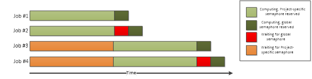
3.5.2. Creating the Project
To create the computational Project, change your current working directory in your R environment to the directory that contains the example material relevant to this example.
After having browsed to the correct directory, you can source the Local Control Code using command:
source("run_semaphore.r")
After having sourced the file, create the computational Project using command:
res <- run_runsemaphore()
Please note that the output generated by the program will change based on whether or not the global semaphore named globalsema is available. The two example screenshots below illustrate the output in both scenarios.
Please also note that there might be overlap in the reported time windows. This is because the time windows are measured from the timestamp generated at the start of the code, which means that e.g. initialization delays can cause the reported times to overlap.
The example screenshot below illustrates the generated output when the global semaphore exists.
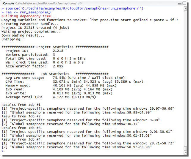
The example screenshot below illustrates the generated output when the global semaphore does not exist.
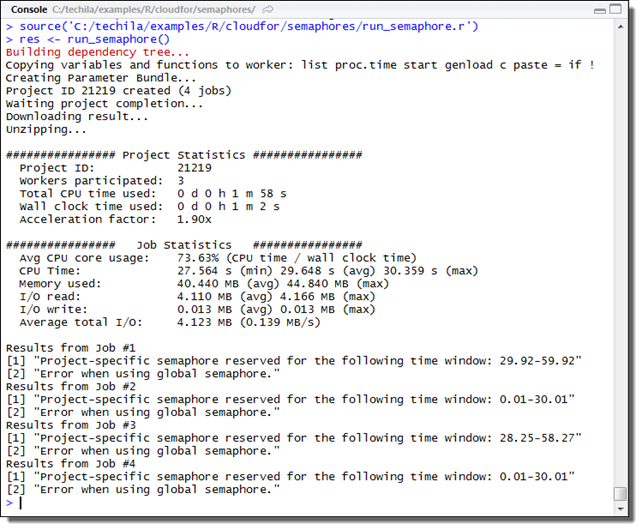
4. Peach Tutorial Examples
This Chapter contains four minimalistic examples on how to implement and control the core features of the peach function. The example material discussed in this Chapter, including R scripts and data files can be found in the subdirectories under the following folder in the Techila SDK:
techila\examples\R\Tutorial
Each of the examples contains three pieces of code:
-
A locally executable R script. The locally executable script can be executed locally and will not communicate with the distributed computing environment in any way. This script is provided as reference material to illustrate what modifications are required to execute the computations in the Techila Distributed Computing Engine (TDCE) environment.
-
A script containing the Local Control Code, which will be executed locally and will be used to distribute the computations in the Techila Worker Code to the distributed computing environment
-
A script containing the Techila Worker Code, which will be executed on the Techila Workers. This script contains the computationally intensive part of the locally executable script.
Please note that the example material in this Chapter is only intended to illustrate the core mechanics related to distributing computation with peach. More information on available features can be found in Peach Feature Examples and by executing the following commands in R.
library(techila)
?peach
4.1. Executing an R Function on the Techila Workers
This example is intended to provide an introduction on distributed computing using TDCE with R using the `peach`function. The purpose of this example is to:
-
Demonstrate how to modify a simple, locally executable R script that contains one function so the computational operations can be performed in the TDCE environment
-
Demonstrate the difference between Local Control Code and Techila Worker Code in R environment
-
Demonstrate the basic syntax of the
peachfunction in R environment
The material discussed in this example is located in the following folder in the Techila SDK:
techila\examples\R\Tutorial\1_distribution
4.1.1. Locally executable R function
The locally executable R script called local_function.r contains one function called local_function, which consists of one for loop. The algorithm of the locally executable function used in this example is shown below.
# Example documentation: http://www.techilatechnologies.com/help/r_tutorial_1_distribution
# Copyright Techila Technologies Ltd.

# This function contains the locally executable function, which can be
# executed on the End-Users computer. This function does not
# communicate with the Techila environment.
#
# Usage:
# source("local_function.r")
# result <- local_function(x)
# x: the number of iterations in the for loop.
#
# Example:
# result <- local_function(5)

local_function <- function(x) {
 result <- array(0, dim = c(1, x))
 for (j in 1:x)
 result[1, j] <- 1 + 1
 result
}
The program requires one input parameter, which defines the number of iterations that will be performed in the for loop. Every iteration performs the same arithmetic operation: 1+1. The result of the latest iteration will get appended to the result vector. The result vector for three iterations is shown below.
loops=3 |
|||
index |
1 |
2 |
3 |
result |
2 |
2 |
2 |
To execute the function, please source the R code using command:
source("local_function.r")
After the R script has been sourced, the function can be executed using command:
local_function(3)
After executing the function, the numerical values stored in the result variable will be displayed.
4.1.2. Distributed version of the program
All arithmetic operations in the locally executable function are performed in the for loop. There are no recursive data dependencies between iterations, meaning that the all the iterations can be performed simultaneously. This is done by placing the computational instructions in the Techila Worker Code (distribution_dist.r).
Local Control Code in the R script run_distribution.r is used to create the computational Project. The Techila Worker Code in the distribution_dist.r file is transferred to the Techila Workers where script will automatically be sourced at the preliminary stages of the Job. After the R script has been sourced, the function distribution_dist will be executed.
4.1.3. Local Control Code
The Local Control Code used to control the distribution process is shown in below.
# Example documentation: http://www.techilatechnologies.com/help/r_tutorial_1_distribution
# Copyright Techila Technologies Ltd.

# This function contains the Local Control Code, which will create the
# computational Project.
#
# Usage:
# source("run_distribution.r")
# result <- run_distribution(jobs)
# jobs: the number of Jobs in the Project
#
# Example:
# result <- run_distribution(5)
run_distribution <- function(jobs) {

  # Load the techila library
  library(techila)

  # Create the computational Project with the peach function.
  result <- peach(funcname = "distribution_dist",    # Function that will be called on Workers
                  files = list("distribution_dist.r"), # R-file that will be sourced on Workers
                  peachvector = 1:jobs,                 # Number of Jobs in the Project
                  sdkroot = "../../../..")              # Location of the techila_settings.ini file

  # Display results after the Project has been completed. Each element
  # will correspond to a result from a different Job.
  print(as.numeric(result))
  result
}
The script defines one function called run_distribution, which requires one input parameter. This input parameter will be used to specify the number of Jobs into which the Project should be split. This will be further done by using the jobs input parameter, which defines the length of the peachvector.
In this example, no input arguments are required by the function that will be executed on the Techila Workers. This means that the params parameter does not need to be defined.
At the final stages of the code, as soon as the results have been transferred back to the End-User’s local computer, the results will be converted to numeric format.
4.1.4. Techila Worker Code
The Techila Worker Code that performs the computations is shown below.
# Example documentation: http://www.techilatechnologies.com/help/r_tutorial_1_distribution
# Copyright Techila Technologies Ltd.

# This function contains the function that will be executed during
# computational Jobs. Each Job will perfom the same computational
# operations: calculating 1+1.
distribution_dist <- function() {

  # Store the sum of 1 + 1 to variable 'result'
  result <- 1 + 1

  # Return the value of the 'result' variable. This value will be
  # returned from each Job and the values be displayed on the
  # End-Users computer after the Project is completed.
  return(result)
}
Operations performed in the Techila Worker Code are equivalent to one iteration of the locally executable loop structure. As no input parameters will be transferred to the Techila Worker Code, identical arithmetic operations are performed during all Jobs. The interaction between the Local Control Code and the Techila Worker Code is illustrated in the image below.
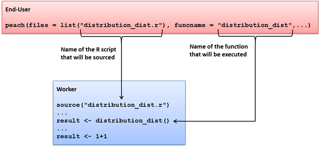
files parameter. In this example, the file distribution_dist.r will be transferred to all Techila Workers and sourced at the preliminary stages of the computational Job. The name of the function that will be called is defined with the funcname parameter. In this example, the function distribution_dist will be called in each computational Job.4.1.5. Creating the computational Project
To create the computational Project, please change your current working directory in your R environment to the directory containing the example material for this example.
After having browsed to the correct directory, you can source the Local Control Code using command:
source("run_distribution.r")
After having sourced the R script, execute the function using command:
result <- run_distribution(3)
This will create a computational Project consisting of three Jobs. Each of the Jobs will be extremely short, as each Job consists of simply summing up two integers; 1+1. The computations occurring during the computational Project are illustrated in the image below:
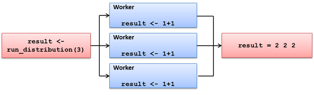
run_distribution is used to determine the number of Jobs. The same arithmetic operation, 1+1, is performed in each Job. Results are delivered back to the End-Users computer where they will be stored in the result vector.4.2. Using Input Parameters
This purpose of this example is to demonstrate:
-
How to give input parameters to the executable function
In this example, parameters will be transferred to the Techila Workers using the params parameter of the peach function. The params parameter can be used to transfer static parameters that are identical across all Jobs or to transfer elements of the peachvector.
The material used in this example is located in the following folder in the Techila SDK:
techila\examples\R\Tutorial\2_parameters
4.2.1. Locally executable R function
The algorithm for the locally executable function used in this example is shown below.
# Example documentation: http://www.techilatechnologies.com/help/r_tutorial_2_parameters
# Copyright Techila Technologies Ltd.

# This function contains the locally executable function, which
# can be executed on the End-Users computer. This function
# does not communicate with the Techila environment.
#
# Usage:
# source("local_function.r")
# result <- local_function(multip, loops)
# multip: value of the multiplicator
# loops: the number of iterations in the 'for' loop.
#
# Example:
# result <- local_function(2, 5)
local_function <- function(multip, loops) {
  result <- 0
  for (x in 1:loops) {
    result[x] <- multip * x
  }
  print(result)
  result
}
This function requires two input parameters; multip and loops. The parameter loops determines the number of iterations in the for loop. The parameter multip is a number, which will be multiplied with the iteration number represented by x. The result of this arithmetic operation will then be appended to a vector called result, which will be returned as the output value of the function. The result vector in a case of five iterations is shown below.
| multip = 2; loops=5 | |||||
|---|---|---|---|---|---|
index |
1 |
2 |
3 |
4 |
5 |
result |
2 |
4 |
6 |
8 |
10 |
To execute the function, please source the R code using command:
source("local_function.r")
As soon as the R script has been sourced, the function can be executed using the command shown below:
local_function(2,5)
After executing the function, numerical values stored in the result variable will be displayed. If you executed the function using the input parameters shown above, the following values will be printed:
[1] 2 4 6 8 10
4.2.2. Distributed version of the program
All the computations in locally executable R script are performed in the for loop and there are no dependencies between the iterations. Because of this, the locally executable program can be converted to a distributed version by extracting the arithmetic operation into a separate piece of code. Input parameters for the executable R function will be transferred with the params array of the peach function.
4.2.3. Local Control Code
The Local Control Code used to control the distribution process is shown in below.
# Example documentation: http://www.techilatechnologies.com/help/r_tutorial_2_parameters
# Copyright Techila Technologies Ltd.

# This function contains the Local Control Code, which will create the
# computational Project.
#
# Usage:
# source("run_parameters.r")
# result <- run_parameters(multip, jobs)
# multip: value of the multiplicator
# jobs: the number of iterations in the 'for' loop.
#
# Example:
# result <- run_parameters(2, 5)

run_parameters <- function(multip, jobs) {

  # Load the techila library
  library(techila)

  # Create the computational Project with the peach function.
  result <- peach(funcname = "parameters_dist",  # Function that will be called on Workers
                  params = list(multip, "<param>"), # Parameters for the function that will be executed
                  files = list("parameters_dist.r"),  # Files that will be sourced at the preliminary stages
                  peachvector = 1:jobs, # Number of Jobs. Peachvector elements will also be used as input parameters.
                  sdkroot = "../../../..") # The location of the techila_settings.ini file.

  # Convert results to numeric format.
  result <- as.numeric(result)
  # Display the results after the Project is completed
  print(result)
  result
}
The function run_parameters requires two input parameters multip and jobs. The multip parameter is listed in the params array, meaning it will be transferred to Techila Workers and given as the first input argument to the executable function.
The jobs parameter is used to define the length of the peachvector, meaning the value of the jobs parameter will define the number of Jobs in the Project. Elements of the peachvector will also be given as the second input argument to the executable function. This is because the second entry in the params parameter is the "<param>" notation, which will automatically be replaced with a different peachvector element on the Techila Workers.
4.2.4. Techila Worker Code
The algorithm for the Techila Worker Code is shown below.
# Example documentation: http://www.techilatechnologies.com/help/r_tutorial_2_parameters
# Copyright Techila Technologies Ltd.

# This function contains the function that will be executed during
# computational Jobs. Each Job will multiply the values of the two
# input arguments, 'multip' and 'jobidx'. 'multip' will be same for
# all Jobs, 'jobidx' will receive a different peachvector element.
parameters_dist <- function(multip, jobidx) {

  # Multiply the values of variables 'multip' and 'jobidx
  result <- multip * jobidx

  # Return the value of the 'result' variable from the Job.
  return(result)
}
The Local Control Code discussed earlier defined two parameters in the params parameter. One of these parameters was a static parameter (multip) and the other was a dynamic parameter ("<param>"). In the Techila Worker Code, the static parameter is being represented by a parameter called multip, which will be constant across all Jobs. The dynamic parameter in the Local Control Code is represented by jobidx parameter, which will get replaced by a different element of the peachvector in each Job. As a result we can say that jobidx parameter simulates the iteration number of the locally executable function.
The interaction between the Local Control Code and the Techila Worker Code is illustrated in the image below.
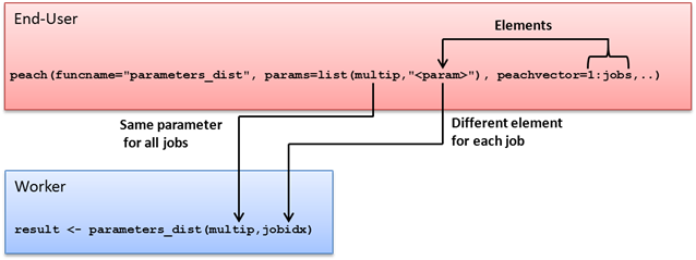
params parameter will be transferred to the function that will be executed on the Techila Workers. The "<param>" notation is used to transfer elements of the peachvector to the Techila Worker Code. The value of the jobs variable is defined by the End-User and it is used to define the length of the peachvector. The value of the jobs parameter therefore defines the number of Jobs.4.2.5. Creating the Project
To create the computational Project, change your current working directory in your R environment to the directory that contains the example material for this example.
After having browsed to the correct directory, you can source the Local Control Code using command:
source("run_parameters.r")
After having sourced the R script, the computational Project can be created using following command:
result <- run_parameters(2,5)
This will create a computational Project that will consist of five Jobs. The parameters in the params parameter in the peach function call will be given values based on the input arguments of the run_parameters function. The Techila Workers will execute the parameter_dist function using one static and one dynamic input parameter.
The static parameter multip to will be set to two (2). The peachvector will contain the integers from one to five. These integers are used to define the value of the jobidx parameter in the Techila Worker Code. The computational operations occurring during the computational Project are illustrated in the image below.
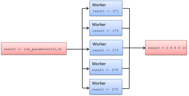
multip parameter is constant, remaining the same for all Jobs. The jobidx parameter is replaced with elements of the peachvector, receiving a different element for each Job. Job results are stored in the result vector in the Local Control Code.4.3. Transferring Data Files
This purpose of this example is to demonstrate:
How to transfer data files
In this example, one file called datafile.txt will be transferred to the Techila Workers using the files parameter of the peach function.
Note that the files parameter should only be used to transfer small files that change frequently. If you plan to transfer large files, or files that will not change frequently, it is advisable that you create a separate Data Bundle to transfer the files. Instructions on how to use a Data Bundle to transfer data files can be found in Data Bundles.
The material used in this example is located in the following folder in the Techila SDK:
techila\examples\R\Tutorial\3_datafiles
4.3.1. Locally executable R function
The locally executable R script used in this example is shown in below.
# Example documentation: http://www.techilatechnologies.com/help/r_tutorial_3_datafiles
# Copyright Techila Technologies Ltd.

# This function contains the locally executable function, which can be
# executed on the End-Users computer. This function does not
# communicate with the Techila environment.
#
# Usage:
# source("local_function.r")
# result <- local_function()
# Example:
# result <- local_function()
local_function <- function() {
  contents <- read.table("datafile.txt")
  n <- length(contents)
  result <- 0
  for (x in 1:n) {
    result[x] <-  sum(contents[1:length(contents), x])
  }
  result
}
During the initial steps of the function, the table in the file datafile.txt will be stored in the contents variable by using the read.table command. The computational part consists of calculating the sum of each column in the table that is stored in the contents variable. The sum of one column is calculated during each iteration.
To execute the function, please source the R code using command:
source("local_function.r")
As soon as the R script has been sourced, the function can be executed using the command shown below:
local_function()
After executing the function, a line will be printed that will display the sums of each column in the table. The printed values should correspond to the values shown below:
[1] 1111 2222 3333 4444
4.3.2. Distributed version of the program
In the distributed version, the file datafile.txt will be transferred to Techila Workers by using the files parameter of the peach function. The values of one column in the table will be summed during one Job.
4.3.3. Local Control Code
The Local Control Code that is used to create the computational Project is shown below.
# Example documentation: http://www.techilatechnologies.com/help/r_tutorial_3_datafiles
# Copyright Techila Technologies Ltd.

# This function contains the Local Control Code, which will create the
# computational Project.
#
# Usage:
# source("run_datafiles.r")
# result <- run_datafiles()
# Example:
# result <- run_datafiles()
run_datafiles <- function()  {

  # Load the techila library
  library(techila)

  # Set the value of the jobs variable to four. The 'jobs' variable
  # will be used to determine the length of peachvector.
  jobs <- 4

  # Create the computational Project with the peach function.
  result <- peach(funcname = "datafiles_dist",  # The function that will be called
                  params = list("<param>"), # Parameters for the executable function
                  files = list("datafiles_dist.r"), # Files that will be sourced on Workers
                  datafiles = list("datafile.txt"),  # Datafiles that will be transferred to Workers
                  peachvector = 1:jobs, # Length of the peachvector determines the number of Jobs.
                  sdkroot = "../../../..") # Location of the techila_settings.ini file.

  # Convert the results to numeric format
  result <- as.numeric(result)
  # Display the results.
  print(result)
  result
}
The function run_data_files requires no input parameters. The number of Jobs in the computational Project will be determined by value of the jobs parameter. This is done by using the jobs parameter to define the length of the peachvector. Elements of the peachvector are also used as a dynamic input parameter in the parameter params as indicated by the "<param>" notation.
The files parameter contains the name of the file (datafile.txt) that will be transferred to all Techila Workers.
4.3.4. Techila Worker Code
The algorithm of the Techila Worker Code used in this example is shown below.
# Example documentation: http://www.techilatechnologies.com/help/r_tutorial_3_datafiles
# Copyright Techila Technologies Ltd.

# This function contains the function that will be executed during
# computational Jobs. Each Job will sum the values in a specific
# column in the file 'datafile.txt' and return the value as the
# output.
datafiles_dist <- function(jobidx) {

  # Read the file 'datafile.txt' from the temporary working directory.
  contents = read.table("datafile.txt")

  # Sum the values in the column. The column is chosen based on the value
  # of the 'jobidx' parameter.
  result = sum (contents[1:length(contents), jobidx])

}
The Local Control Code introduced earlier defines one dynamic input parameter. This is represented in the Techila Worker Code by the jobidx parameter, which will get replaced by a different element of the peachvector in each Job. In Job 1, the value will be one (1), in Job 2, the value will be 2 and so on. This means that the jobidx parameter can be used to point to the correct column during each Job.
The Local Control Code also introduced one (1) filename in the files array. This file will be copied to the same temporary working directory at the Techila Worker with the executable code, which means that the file datafile.txt can be loaded into memory using the same syntax as in a locally executable function.
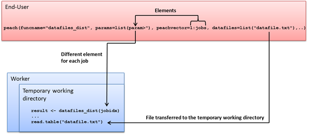
4.3.5. Creating the computational project
To create the computational Project, change your current working directory in your R environment to the directory that contains the example material for this example.
After having browsed to the correct directory, you can source the Local Control Code using command:
source("run_datafiles.r")
After having sourced the R script, execute the function using command:
result <- run_datafiles()
The number of Jobs in the Project will be automatically fixed to four as the value of the jobs parameter is defined in the Local Control Code. Parameters in the params parameter and the file specified in the files parameter will be transferred to the Techila Workers. The function will be executed using the dynamic input parameter and the Techila Workers will access the file specified in the files parameter from the temporary working directory.
4.4. Multiple Functions in an R Script
A locally executable R script can contain a large number of object definitions and/or function calls. In a similar fashion, Techila Worker Code can also contain several functions and/or object definitions. As mentioned earlier in R Peach Function, the R script containing the Techila Worker Code will be sourced with the source command at the beginning of a computational Job. This means that any function that is defined in the R script can also be called by using the name of the function as the value of the funcname parameter.
The material used in this example is located in the following folder in the Techila SDK:
techila\examples\R\Tutorial\4_multiplefunctions
4.4.1. Locally executable R functions
The R script containing the locally executable functions is shown below.
# Example documentation: http://www.techilatechnologies.com/help/r_tutorial_4_multiplefunctions
# Copyright Techila Technologies Ltd.

# This R-script contains two locally executable functions, which
# can be executed on the End-Users computer. These functions
# do not communicate with the Techila environment.

function1 <- function() {
  # When called, this function will return the value 2.
  result <- 1 + 1
}

function2 <- function() {
  # When called, this function will return the value 100.
  result <- 10 * 10
}
To execute the functions on your local computer, please source the R code using command:
source("local_multiple_functions.r")
As soon as the R script has been sourced, function1 function can be executed with command:
result <- function1()
When called, function1 will perform the summation 1+1 and return 2 as the result.
Respectively, the function called function2 can be executed with command:
result <- function2()
When called, function2 will perform the multiplication 10*10 and return 100 as the result.
4.4.2. Distributed version of the program
In this example, the functions in the locally executable R script will be placed directly into the R script containing the Techila Worker Code (multi_function_dist.r).
Local Control Code in the R script (run_multi_function.r) is used to create the computational Project. The funcname parameter in the peach function call determines which function will be called from the functions defined in the Techila Worker Code.
4.4.3. The Local Control Code
The Local Control Code used to create the computational Project is shown below.
# Example documentation: http://www.techilatechnologies.com/help/r_tutorial_4_multiplefunctions
# Copyright Techila Technologies Ltd.

# This function contains the Local Control Code, which will create the
# computational Project. The value of the input argument will
# determine which function will be executed in the computational Jobs.
#
# Usage:
# source("run_multi_function.r")
# result <- run_multi_function(funcname)
# Example:
# result <- run_multi_function("function1")

run_multi_function <- function(funcname) {

  # Load the techila library
  library(techila)

  # Create the computational Project with the peach function.
  result <- peach(funcname = funcname, # Executable function determined by the input argument of 'run_multi_function'
                  files = list("multi_function_dist.r"), # The R-script that will be sourced on Workers
                  peachvector = 1:1, # Set the number of Jobs to one (1)
                  sdkroot = "../../../..") # Location of the techila_settings.ini file

  # Convert the results to numeric format and display them.
  print(as.numeric(result))
}
The function run_multi_function requires one input parameter. This input parameter is used to determine, which function will be called during a Job. This is performed by setting the value of the funcname parameter to the value of the input parameter.
4.4.4. Techila Worker Code
The Techila Worker Code ("multi_function_dist.r") used in this example is shown below.
# Example documentation: http://www.techilatechnologies.com/help/r_tutorial_4_multiplefunctions
# Copyright Techila Technologies Ltd.

# This R-script will be sourced at the preliminary stages of a
# computational Job. The value of input argument in the Local Control
# Code will determine, which function will be called on the Worker.

function1 <- function() {
  # When called in the computational Job, the function return the value 2.
  result <- 1 + 1
}

function2 <- function() {
  # When called in the computational Job, the function return the value 100.
  result <- 10 * 10
}
As can be seen, the Techila Worker Code contains the same function definitions as the locally executable R script. The Techila Worker Code will be sourced at the preliminary stages of a computational Job, meaning both functions will be defined during a computational Job. This means either function can be called by with the funcname parameter in the Local Control Code.
4.4.5. Creating the computational Project
To create the computational Project, change your current working directory (in R) to the directory that contains the example material relevant to this example.
After having browsed to the correct directory, you can source the Local Control Code using command:
source("run_multi_function.r")
After having sourced the Local Control Code, a computational Project that executes function1 on Techila Workers can be created using command shown below:
result <- run_multi_function("function1")
This will create a computational Project that consists of one (1) Job. The computational operations occurring during the Project are illustrated in the image below.
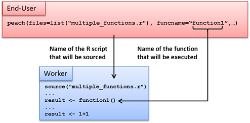
Respectively, function2 can be executed on the Techila Worker by using the command:
result <- run_multi_function("function2")
The computational operations occurring during the Projects are illustrated in the image below.
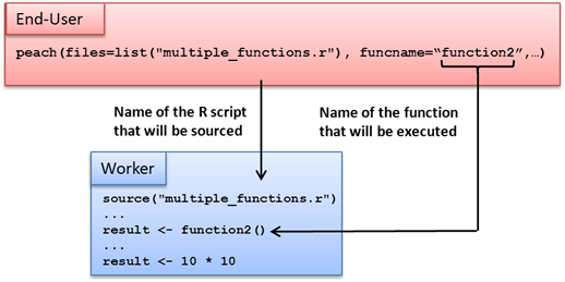
5. Peach Feature Examples
The basic methodology and syntax of distributing computations using R peach was shown in the Tutorial in Peach Tutorial Examples. In addition to the features used in the Tutorial, peach offers a wide range of optional features.
This Chapter will consist of examples on implementing some of the advanced features available in peach. The implementations are demonstrated using the approximation of 𝜋 using Monte Carlo methods as a framework. Peach Feature Examples contains the basic implementation of approximating the value of Pi with the Monte Carlo method.
The example material used this Chapter, including R scripts and data files can be found in the subdirectories under the following folder in the Techila SDK:
techila\examples\R\Features\<example specific subfolder>
Please note that the example material discussed in this Chapter does not contain examples on all available peach features. For a complete list on available features, execute the following command in R:
library(techila)
?peach
Monte Carlo Method
A Monte Carlo method is used in several of the examples for evaluating the value of Pi. This section contains a short introduction on the Monte Carlo method used in these examples.
The Monte Carlo method is a statistical simulation where random numbers are used to model and solve a computational problem. This method can also be used to approximate the value of Pi with the help of a unit circle and a random number generator.
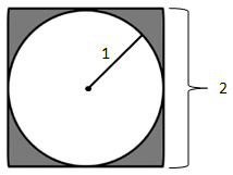
The area of the unit circle shown in the figure is determined by the equation π∙r^2 and the area of the square surrounding it by the equation (2 * r)^2. This means the ratio of areas is defined as follows:
ratio of areas = (area of the unit circle)/(area of the square) = (pi * r ^ 2 /( (2 * r) ^2 )=( pi * r ^ 2 / (4 * r ^ 2 )= pi / 4 = 0.7853981
When a random point will be generated, it can be located within or outside the unit circle. When a large number of points are being generated with a reliable random number generator, they will be spread evenly over the square. As more and more points are generated, the ratio of points within circle compared to the total number of points starts to approximate the ratio of the two areas.
ratio of points * ratio of areas
(points within the circle)/(total number of points) = (area of the unit circle)/(area of the square)
(points within the circle)/(total number of points) = pi / 4
For example, in a simulation of 1000 random points, the typical number of points within the circle is approximately 785. This means that the value of Pi is calculated in the following way.
785 / 1000 * pi / 4
pi * 4 * 785 / 1000 = 3.14
Algorithmic approaches are usually done only using one quarter of a circle with a radius of 1. This is simply because of the fact that number generating algorithms on many platforms generate random numbers with a uniform(0,1) distribution. This does not change the approximation procedure, because the ratios of the areas remain the same.
5.1. Monte Carlo Pi with Peach
This example will demonstrate:
-
Approximation of the value of Pi using Monte Carlo method
-
Converting a locally implemented Monte Carlo method to a distributed version
The material used in this example is located in the following folder in the Techila SDK:
techila\examples\R\Features\basic_monte_carlo_pi
5.1.1. Locally executable function
The locally executable function for approximating the value of Pi used in this example is shown below.
# Example documentation: http://www.techilatechnologies.com/help/r_features_basic_monte_carlo_pi
# Copyright Techila Technologies Ltd.

# This function contains the locally executable function, which can be
# executed on the End-Users computer. This function does not
# communicate with the Techila environment. The function implements a
# Monte Carlo routine, which approximates the value of Pi.
#
# Usage:
# source("local_function.r")
# result <- local_function(mloops)
# loops: the number of iterations in Monte Carlo approximation
#
# Example:
# result <- local_function(100000)

local_function <- function(loops){

  # Initialize counter to zero.
  count <- 0

  # Perform the Monte Carlo approximation.
  for (i in 1:loops) {
    if ((sum(((runif(1) ^ 2)  + (runif(1) ^ 2))) ^ 0.5) < 1) { # Calculate the distance of the random point
     count <- count + 1  # Increment counter, when the point is located within the unitary circle.
    }
  }
  # Calculate the approximated value of Pi based on the generated data.
  pivalue <- 4 * count / loops
  # Display results
  print(c("The approximated value of Pi is:", pivalue))
  pivalue
}
The local_function-function requires one input argument called loops, which determines the number of iterations in the for loop. During each iteration, two random numbers will be generated, which will be used as the coordinates of the random point. The coordinates of the point are then used to calculate the distance of the point from the centre of the unit circle. If the distance is less than one, the point is located within the unit circle and the counter is incremented by one. As soon as all iterations have been completed, the value of Pi will be calculated.
To execute the locally executable function that approximates the value of Pi, source the R code using command:
source("local_function.r")
As soon as the R code has been sourced, the function can be executed using command:
local_function(10000000)
This will approximate the value of Pi using 10,000,000 randomly generated points. The operation will take approximately five minutes, depending on the speed of your CPU. If you wish to perform a shorter approximation, reduce the number of random points generated to e.g. 1000000.
After the approximation is completed, the approximated value of Pi will be displayed in the R Console as shown below.
"The approximated value of Pi is:" "3.141396"
Note that due to randomness of the Monte Carlo method, the last decimals in your result will likely differ from the one shown above.
5.1.2. Distributed version of program
The computationally intensive part in Monte Carlo methods is the random number sampling, which is performed in the for loop in the locally executable function. There are no dependencies between the iterations. This means that the sampling process can be divided into a separate function and executed simultaneously on several Techila Workers.
Note that the seed of the random number generator is initialized automatically on the Techila Workers by the peachclient as explained in R Peach Function. If you wish to use a different seeding method, please seed the random number generator directly in the Techila Worker Code.
5.1.3. Local Control Code
The Local Control Code used in this example to create the computational Project is shown below.
# Example documentation: http://www.techilatechnologies.com/help/r_features_basic_monte_carlo_pi
# Copyright Techila Technologies Ltd.

# This R-script contains the Local Control Code, which will be used to
# distribute computations to the Techila environment.
#
# The R-script named "mcpi_dist.r" will be distributed and sourced on
# Workers. The 'loops' parameter will be transferred to all Jobs. The
# peachvector will be used to control the number of Jobs in the
# Project. The 'run_mcpi' function will return the value of the
# 'result' variable, which will contain the approximated value of Pi.
#
# Usage:
# source("run_mcpi.r")
# result <- run_mcpi(jobs, loops)
# jobs: number of Jobs in the Project
# loops: number of Monte Carlo approximations performed per Job
#
# Example:
# result <- run_mcpi(10, 100000)

# Load the techila library
library(techila)

run_mcpi <- function(jobs, loops) {

  # Create the computational Project with the peach function.
  result <- peach(funcname = "mcpi_dist", # Function that will be executed on Workers
                  params = list(loops), # Parameters for the executable function
                  files = list("mcpi_dist.r"), # Files that will be sourced on Workers
                  peachvector = 1:jobs, # Length of the peachvector determines the number of Jobs.
                  sdkroot = "../../../..") # Location of the techila_settings.ini file

  # Calculate the approximated value of Pi based on the generated data.
  result <- 4 * sum(as.numeric(result)) / (jobs * loops)

  # Display results
  print(c("The approximated value of Pi is:", result))
  result
}
The first line of the Local Control code consists of loading the techila library by using the library(techila) command. The line containing the peach function call is responsible for distributing the computations to the distributed computing environment. After the peach function returns, individual results from Jobs will be combined and used to calculate the approximate value of Pi.
5.1.4. Techila Worker Code
The code that is executed on Techila Workers in this example is shown below.
# Example documentation: http://www.techilatechnologies.com/help/r_features_basic_monte_carlo_pi
# Copyright Techila Technologies Ltd.

# This R-script contains the Worker Code, which will be distributed
# and sourced on the Workers. The values of the input parameters will
# be received from the parameters defined in the Local Control Code.
mcpi_dist <- function(loops) {

  count <- 0 # No random points generated yet, init to 0.
  for (i in 1:loops) { # Monte Carlo loop from 1 to loops
    if ((sum(((runif(1) ^ 2)  + (runif(1) ^ 2))) ^ 0.5) < 1) { # Point within the circle?
     count <- count + 1  # Increment if the point is within the circle.
    }
  }
  return(count) # Return the number of points within the unitary circle
}
The algorithm is very similar to the algorithm of the locally executable function. The function requires one input argument called loops which is being used to determine the number of iterations. Every iteration calculates the distance of a randomly generated point from the centre. If the distance is less than one, the point is within the unit circle and the count is incremented by one. No post-processing activities are performed in the Techila Worker Code, as the results from individual Jobs are post-processed in the Local Control Code.
5.1.5. Creating the computational project
To create the computational Project, change your current working directory to the directory containing the example material. Source the Local Control Code using command:
source("run_mcpi.r")
As soon as the R script has been sourced, please execute the function using command:
result <- run_mcpi(10,1000000)
This will create a Project consisting of ten Jobs, each containing 1,000,000 iterations. The Jobs will be distributed to Techila Workers, where the Monte Carlo routine in the Techila Worker Code is executed. When a Techila Worker finishes the Monte Carlo routine, results are transferred to the Techila Server. After all the Techila Workers have transferred the results to the Techila Server, the results are transferred to the End-Users computer. After the results have been downloaded, the last line in the control code is executed which contains the post-processing operations, which in this case consist of scaling the results according to the number of performed iterations.
5.2. Streaming & Callback Function
Streaming enables individual results to be transferred as soon as they become available. This is different from the default implementation, where all the results will be transferred in a single package after all of the Jobs have been completed.
The Callback function enables results to be handled as soon as they have been streamed from the Techila Server to End-User. The Callback function is called once for each result file that will be transferred from the Techila Server. The example presented in this Chapter uses Streaming and Callback functions.
The material used in this example is located in the following folder in the Techila SDK:
techila\examples\R\Features\streaming_callback
Streaming is disabled by default. Streaming can be enabled with the following parameter pair:
stream = TRUE
A function can be used as a Callback function by defining the name of the function using the following parameter pair:
callback="<callback function name>"
The notation <callback function name> would be replaced with the name of the function you wish to use.
The callback function will then be called every time a new result file has been streamed from the Techila Server to End-User. The callback function will receive a single input argument, which will contain the result returned from the Techila Worker Code.
Values returned by the callback function will be the values of the peach result vector. Since new values are appended to the result vector in the order in which Jobs are being completed, values in the result vector will be in a random order.
The implementation of the Streaming and Callback features will be demonstrated using the Monte Carlo Pi method. In the distributed version of the program, Job results will be streamed as soon as they have become available. The callback function is used to print the approximated value of P in a continuous manner.
5.2.1. Local Control Code
The Local Control Code of the Monte Carlo Pi where Callback function and Streaming are used is shown below.
# Example documentation: http://www.techilatechnologies.com/help/r_features_streaming_callback
# Copyright Techila Technologies Ltd.

# This R-script contains the Local Control Code, which will be used to
# distribute computations to the Techila environment.
#
# The R-script named "mcpi_dist.r" will be distributed to Workers,
# where the function mcpi_dist will be executed according to the
# defined input parameters.
#
# The peachvector will be used to control the number of Jobs in the
# Project.
#
# Results will be streamed from the Workers in the order they will be
# completed. Results will be visualized by displaying intermediate
# results on the screen.
#
# To create the Project, use command:
#
# result <-  run_streaming(jobs,loops)
#
# jobs = number of jobs
# loops = number of iterations performed in each Job

# Load the techila library
library(techila)

# Create a global variable to store intermediate results.
total<-new.env()

# This is the callback functions, which will be executed once for each
# Job result received from the Techila environment.
callbackFun <- function(result) {

  total$jobs <- total$jobs + 1 # Update the number of Job results processed
  total$loops <- total$loops + result$loops # Update the number of Monte Carlo loops performed
  total$count <- total$count + result$count # Update the number of points within the unitary circle
  result <- 4 * total$count / total$loops # Update the Pi value approximation

  # Display intermediate results
  print(paste("Number of results included:",total$jobs," Estimated value of Pi:",result))
  result
}

# When executed, this function will create the computational Project
# by using peach.
run_streaming <- function(jobs,loops) {

  # Initialize the global variables to zero.
  total$jobs <- 0
  total$loops <- 0
  total$count <- 0

  result <- peach(funcname = "mcpi_dist", # Name of the executable function
                  params = list(loops), # Input parameters for the executable function
                  files = list("mcpi_dist.r"), # Files for the executable function
                  peachvector = 1:jobs, # Length of the peachvector will determine the number of Jobs in the Project
                  sdkroot = "../../../..", # Location of the techila_settings.ini file
                  stream = TRUE, # Enable streaming
                  callback = "callbackFun" # Name of the callback function
                 )
}
The Local Control Code here consists of two functions, run_streaming and callbackFun. The run_streaming function will distribute the computations using peach. The function called callbackFun is the callback function that will be executed every time a new result will be streamed from the Techila Server to the End-User’s computer. The variables used in the callback function are declared as global to preserve the values of the parameters between function calls. The input argument of the callback function (result) will be replaced by the result returned from the Techila Worker Code.
The Callback function callbackFun contains the arithmetic operations to continuously update the approximated value of Pi. The value will be printed in a continuous manner as results are received from the Techila Server. The Callback function will return the approximated value of Pi, based on the results received so far. This approximated value will be stored in the result vector returned by peach.
5.2.2. Techila Worker Code
The Techila Worker Code used in this example is shown below.
# Example documentation: http://www.techilatechnologies.com/help/r_features_streaming_callback
# Copyright Techila Technologies Ltd.

# This R-script contains the Worker Code, which will be distributed and sourced
# on the Workers. The values of the input parameters will be received from the
# parameters defined in the Local Control Code.
mcpi_dist <- function(loops) {

  count <- 0 # No random points generated yet, init to 0.
  for (i in 1:loops) { # Monte Carlo loop from 1 to loops
    if ((sum(((runif(1) ^ 2)  + (runif(1) ^ 2))) ^ 0.5) < 1) { # Point within the circle?
      count <- count + 1 # Increment if the point is within the circle.
    }
  }
  return(list(count=count,loops=loops)) # Return the results as a list
}
The code is similar to the basic implementation introduced in Monte Carlo Pi with Peach, the differentiating factor is that both the count and loops variables are returned in a list. This means that the callback function callbackFun in the Local Control Code will receive the list as the input argument.
5.2.3. Creating the computational project
To create the computational Project, change your current working directory (in R) to the directory that contains the example material relevant to this example.
After having browsed to the correct directory, you can source the Local Control Code using command:
source("run_streaming.r")
After having sourced the R script, execute the function using command:
run_streaming(20,100000)
This will create a computational Project consisting of 20 Jobs, each Job performing a Monte Carlo routine that consists of 100,000 iterations. Results will be streamed from the Techila Server to End-User as they are completed and the approximated value continuously as more results are streamed.
5.3. Job Input Files
Job Input Files allow using Job-specific input files and can be used in scenarios, where individual Jobs require only access to some files within the dataset. Job-Specific Input Files are stored in a Job Input Bundle and will be transferred to the Techila Server. Techila Server will transfer files from the Bundle to the Techila Workers requiring them. These files will be stored on the Techila Worker for the duration of the Job. The Job-Specific input files will be removed from the Techila Worker as soon as the Job has completed.
The material used in this example is located in the following folder in the Techila SDK:
techila\examples\R\Features\job_input_files
The names of Job-specific input files are defined in the jobinputfiles parameter. The parameter contains two named parameters; datafiles and filenames.
-
datafiles is used to determine, which files are transferred to Techila Workers.
-
filenames determines the names of the files after they have been transferred to the Techila Workers
An example of the jobinputfiles parameter is shown below:
jobinputfiles = list(
                datafiles = list("file_1_for_job_1","file_1_for_job_2"),
                filenames = list("worker_file")
                  )
The syntax shown above assigns one Job-Specific input file for each of the two Jobs. The files will be renamed to worker_file at the preliminary stages of each Job.
Several Job-specific input files can be associated with each Job by using a similar syntax as shown below:
jobinputfiles = list(
                  datafiles = list(
                   list("file_1_for_job_1", " file_2_for_job_1"),
                   list("file_1_for_job_2", " file_2_for_job_2")
   )
 filenames = list(
   list("worker_file_1", "worker_file_2")
   )
The syntax shown above assigns two Job-Specific inputs file for each of the two Jobs. The files will be renamed to worker_file_1 and worker_file_2 at the preliminary stages of each Job.
Note! When using Job-specific input files, the number of list elements in the datafiles parameter must be equal to the number of Jobs in the Project.
The use of Job input Files is illustrated using four text files. Each of the text files contains a table of numerical values, which will be summed and the value of the sum will be returned as the result. The computational work performed in this example is trivial and is only intended to illustrate the mechanism of using Job-Specific Input Files.
5.3.1. Local Control Code
The Local Control Code for creating a project that uses Job-Specific Input Files is shown below.
# Example documentation: http://www.techilatechnologies.com/help/r_features_job_input_files
# Copyright Techila Technologies Ltd.

# This function contains the Local Control Code, which will be used to
# distribute computations to the Techila environment.
#
# The R-script named "inputfiles_dist" will be distributed and
# executed on Workers. Job specific input files will be transferred
# with each Job, each Job receiving one input file.
#
# To create the Project, use command:
#
# result <- run_inputfiles()
#
# Note: The number of Jobs in the Project will be automatically set to
# four.

# Load the techila library
library(techila)

run_inputfiles <- function() {

  # Set the number of jobs to four
  jobs <- 4

  result <- peach(funcname = "inputfiles_dist", # Name of the executable function
                  files = list("inputfiles_dist.r"), # Files that will be sourced on Workers
                  peachvector = 1:jobs, # Length of the peacvector determines the number of jobs; in this example four (4)
                  sdkroot = "../../../..", # Location of the techila_settings.ini file
                  jobinputfiles = list(  # Job Input Bundle
                    datafiles = list( # Files for the Job Input Bundle
                      "input1.txt",  # File input1.txt for Job 1
                      "input2.txt", # File input2.txt for Job 2
                      "input3.txt", # File input3.txt for Job 3
                      "input4.txt"  # File input4.txt for Job 4
                    ),
                    filenames = list("input.txt") # Name of the file on the Worker side
                  )
                 )
}
The datafiles parameter in the jobinputfiles parameter specifies which files should be used in each Job. The syntax used in this example is shown below:
datafiles = list("input1.txt",
                 "input2.txt",
                 "input3.txt",
                 "input4.txt")
) This syntax assigns one input file for each Job. The file `input1.txt` will be transferred to a Techila Worker with Job 1, file `input2.txt` is transferred with Job 2 and so on. Note that the number of entries in the list is equal to the number of elements in the peachvector.
The filenames parameter in the jobinputfiles parameter specifies the names of the files after they have been transferred to the Techila Worker. The syntax used in this example is shown below:
filenames = list("input.txt")This syntax assigns the name input.txt to all Job-Specific Input Files.
5.3.2. Techila Worker Code
Techila Worker Code used to perform operations on the Job-specific input files is shown below.
# Example documentation: http://www.techilatechnologies.com/help/r_features_job_input_files
# Copyright Techila Technologies Ltd.

# This function contains the Worker Code, which will be distributed
# and executed on the Workers. The Jobs will access their Job-specific
# input files with the name "input.txt", which is defined in the Local
# Control Code
inputfiles_dist <- function() {
  table_contents <- read.table("input.txt")
  result <- sum(table_contents)
  return(result)
}
In this example, all the Jobs access their input files by using the file name input.txt. Each Techila Worker then sums the numbers in the Job-specific input file. The value of the summation will be returned as the result.
5.3.3. Creating the computational project
To create the computational Project, change your current working directory in your R environment to the directory that contains the example material for this example.
After having browsed to the correct directory, you can source the Local Control Code using command:
source("run_inputfiles.r")
After having sourced the R script, execute the function using command:
result <- run_inputfiles()
This will create a Project consisting of four Jobs. The system will automatically assign a Job-Specific Input File to each Job, according to the jobinputfiles parameter in the Local Control Code. This is illustrated in the image below.
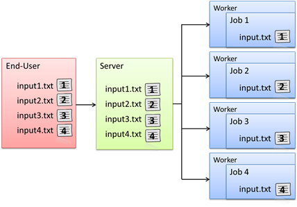
5.4. Project Detaching
When a Project is detached, the peach function returns immediately after all of the computational data has been transferred to the Techila Server. This means that R does not remain in "busy" state for the duration of the Project and can be used for other purposes while the project is being computed. Results of a Project can be downloaded after the Project has been completed by using the Project ID number.
The material used in this example is located in the following folder in the Techila SDK:
techila\examples\R\Features\detached_project
Projects can be detached using following parameter:
donotwait = TRUE
This will cause the peach function to return immediately after the Project has been created and all computational data transferred to the Techila Server. The peach function will return the Project ID number, which can be used in the download process.
Results can be downloaded by linking the peach function call to an existing Project ID number using following parameter pair:
projectid = <project ID number>
It is also possible to download results of a previously completed Project, even when the original Project was not detached with the donotwait parameter. Results belonging to such Projects can be downloaded by defining the Project ID number as the value of the projectid parameter.
Note that results can only be downloaded from the Techila Server if they have not been marked for removal. Removal of Project results can be disabled with the following parameter pair.
removeproject = FALSE
Project ID numbers of previously completed Projects can be viewed from the Techila Web Interface.
The following example demonstrates how to detach a Project and download results using peach.
5.4.1. Local Control Code
The Local Control Code in the run_detached.r script contains two functions, which can be used for creating the detached Project and for downloading the results.
# Example documentation: http://www.techilatechnologies.com/help/r_features_detached_project
# Copyright Techila Technologies Ltd.

# This file contains the Local Control Code, which contains two
# functions:
#
# * run_detached - used to create the computational Project.
# * download_result - used to download the results
#
# The run_detached function will return immediately after all
# necessary computational data has been transferred to the server. The
# function will return the Project ID of the Project that was created.
# The donwnload_result function can be used to download Project
# results by using Project ID number.
#
# Usage:
# Source with command:
# source("run_detached.r")
# Create Project with command:
# projectid <- run_detached(jobs,loops)
# Download results with command:
# result <- download_result(projectid)
#
# jobs = number of jobs
# loops = number of iterations performed in each Job

# Load the techila library
library(techila)

run_detached <- function(jobs,loops) {

  pid <- peach(funcname = "mcpi_dist", # Function that will be executed on Workers
               params = list(loops), # Input parameters for the executable function
               files = list("mcpi_dist.r"), # Files that will be sourced on Workers
               peachvector = 1:jobs, # Length of the peachvector determines the number of Jobs.
               sdkroot = "../../../..", # Location of the techila_settings.ini file
               donotwait = TRUE # Detach project and return after all computational data has been transferred
              )
}

download_result <- function(pid) {

  result <- peach(projectid = pid, # Link to an existing Project.
                  sdkroot = "../../../..") # Location of the techila_settings ini

  points <- 0 # Initialize result counter to zero

  for (i in 1:length(result)) {  # Process each Job result
    points <- points + result[[i]]$count # Calculate the total number of points within the unitary
  }
  result <- 4 * points / (length(result) * result[[1]]$loops) # Calculate the approximated value of Pi
}
The first peach function call creates a Project and detaches it by using the parameter pair:
donotwait = TRUE
The parameter pair causes the peach function to return after the Project has been created. The Project ID number of the Project will be returned by the peach function and stored in the variable pid. This Project ID number will be used to download results after the Project has been completed.
After the Project has been completed, the results can be downloaded by executing the download_result function.
The peach function call in the download_result function will be used to connect to the Techila Server and request the results. The download request is linked to the previously created project with the following parameter pair:
projectid = pid
The pid parameter will specify the Project ID number of the Project that the results will be downloaded for. The value of the parameter is defined as the input argument of the download_result function. The downloaded results will be post-processed to calculate the approximate value of Pi.
5.4.2. Techila Worker Code
The code that is executed on the Techila Workers is shown below.
The Techila Worker Code performs the same Monte Carlo routine as was performed in the basic Monte Carlo Pi implementation presented in Monte Carlo Pi with Peach.The only difference is that the function returns a list containing the results (variable count) and the number of iterations performed (variable loops).
The number of iterations is stored in order to preserve information that is required in the post-processing. Embedding the variables required in post-processing in the result files means, that the post-processing activities can be performed correctly regardless of when the results are downloaded.
5.4.3. Creating the computational Project
To create the computational Project, change your current working directory in your R environment to the directory that contains the example material relevant to this example.
After having browsed to the correct directory, you can source the Local Control Code using command:
source("run_detached.r")
After having sourced the file, create the computational Project using command:
pid <- run_detached(10,1000000)
This creates a Project consisting of ten Jobs. After all of the computational data has been transferred to the Techila Server, the Project ID number will be returned to the pid variable. The Project ID number can be used to download the results of the Project after all the Project has been completed.
After the Project has been completed, the results can be downloaded from the Techila Server with the download_result function using the syntax shown below:
results <- download_result(pid)
5.5. Iterative Projects
Using iterative projects is not so much as a feature as it is a technique. Projects that require that use the output values of previous projects as input values can be implemented by for example placing the peach function call inside a loop structure.
The material used in this example is located in the following folder in the Techila SDK:
techila\examples\R\Features\iterative_projects
5.5.1. Local Control Code
The Local Control Code used to create several, consecutively created projects is shown below.
# Example documentation: http://www.techilatechnologies.com/help/r_features_iterative_projects
# Copyright Techila Technologies Ltd.

# This R-script contains the Local Control Code, which will be used to
# distribute computations to the Techila environment.
#
# The R-script named "mcpi_dist.r" will be distributed and executed
# Workers. Several consecutive Projects will be created, during which
# the value of Pi will be calculated using the Monte Carlo method.
# Results of the Projects will be used to improve the accuracy of the
# approximation. Projects will be created until the amount of error in
# the approximation is below the threshold value.
#
# To create the Projects, use command:
#
# result <- run_iterative()
#
# Note: The number of Jobs in the Project will be automatically set to
# 20.

library(techila)

run_iterative <- function() {
  threshold <-  0.0003  # Maximum allowed error
  jobs <- 20            # Number of Jobs
  loops <- 1e5          # Number of iterations performed in each Job
  total_result <- 0     # Initial result when no approximations have been performed.
  iteration <- 1        # Project counter, first Project will
  current_error <- pi   # Initial error, no approximations have been performed

  while ( abs(current_error) >= threshold ) {

    result <- peach(funcname = "mcpi_dist", # Function that will be executed
                    params = list(loops, "<param>", iteration), # Input parameters for the executable function
                    files = list("mcpi_dist.r"), # Files that will be sourced on Workers
                    peachvector = 1:jobs, # Length of the peachvector is 20 -> set the number of Jobs to 20
                    sdkroot = "../../../..", # Location of the techila_settings.ini file
                    donotuninit = TRUE,  # Do not uninitialize the Techila environment after completing the Project
                    messages = FALSE # Disable message printing
                   )

    # If result is NULL after peach exits, stop creating projects.
    if (is.null(result)) {
      uninit()
      stop("Project failed, stopping example.")
    }

    total_result <- total_result + sum(as.numeric(result)) # Update the total result based on the project results
    approximated_pi <- total_result * 4 / (loops * jobs * iteration)  # Update the approximation value
    current_error <- approximated_pi - pi   # Calculate the current error in the approximation
    print(paste("Amount of error in the approximation = ", current_error))  # Display the amount of current error
    iteration <-iteration+1 # Store the number of completed projects
  }
  # Display notification after the threshold value has been reached
  print("Error below threshold, no more Projects needed.")
  uninit()
  current_error
}
The peach function call is placed inside a loop structure, which is implemented with a while statement. New computational Projects will be created until the error in the approximation is below the predefined threshold value. The amount of error in the approximation will be printed every time a new Project has been completed. Note that messages have been disabled in order to provide a more clear illustration of the results received from Projects.
If the peach function returns NULL, the example will be stopped and all temporary files will be removed by using the unload command. The unload command will also be automatically executed after all Projects have been completed. The run_iterative-function will return the amount of error in the approximation after all Projects have been completed.
5.5.2. Techila Worker Code
The algorithm for the Techila Worker Code is shown below.
# Example documentation: http://www.techilatechnologies.com/help/r_features_iterative_projects
# Copyright Techila Technologies Ltd.

# This R-script contains the Worker Code, which will be distributed
# and sourced on the Workers. The values of the input parameters will
# be received from the parameters defined in the Local Control Code.
mcpi_dist <- function(loops, jobidx, iteration) {
  set.seed(jobidx * iteration)

  count <- 0 # No random points generated yet, init to 0.
  for (i in 1:loops) { # Monte Carlo loop from 1 to loops
    if ((sum(((runif(1) ^ 2)  + (runif(1) ^ 2))) ^ 0.5) < 1) { # Point within the circle?
      count <- count + 1  # Increment if the point is within the circle.
    }
  }
  return(count) # Return the number of points within the unitarty circle
}
The seed of the random number generator is defined by the values of jobidx and iteration variables. This is simply to ensure that the number of consecutive Projects required stays within a reasonable limit. The computational operations performed in the Techila Worker Code are similar as in the basic implementation presented in Monte Carlo Pi with Peach, returning the number of random points that are located within the unitary circle.
5.5.3. Creating the computation Project
To create the computational Project, change your current working directory (in R) to the directory that contains the example material relevant to this example.
After having browsed to the correct directory, you can source the Local Control Code using command:
source("run_iterative.r")
After having sourced the R script, execute the function using command:
run_iterative()
The command shown above will create projects consisting of 20 Jobs. Each Job will consist of 100,000 iterations. Projects will be created until the error of the approximated value is smaller than the threshold value. The error of the approximation will be printed every time a Project has been completed.
5.6. Data Bundles
Data Bundles can be used to efficiently transfer and manage large amounts of data in computational Projects. After being created, Data Bundles will be stored on the Techila Server from where they will be automatically used in future Projects, assuming that the content of the Data Bundle does not change. If the content of the Data Bundle changes (e.g. new files added, existing files removed or the content of existing files modified), a new Data Bundle will be automatically created and transferred to the Techila Server.
The material used in this example is located in the following folder in the Techila SDK:
techila\examples\R\Features\data_bundle
Data Bundles are created by using the databundle parameter. The syntax shown below stores files called F1_B1 and F2_B1 in to a Data Bundle
databundles = list(list(datafiles = list("F1_B1","F2_B1")))An expiration period can be defined for the Data Bundle, which will determine the time period how long an unused Bundle will be stored on a Techila Worker. If a value is not defined, the default expiration periods will be used. For example, an expiration period of 60 minutes can be defined with the following syntax:
databundles = list(list(datafiles = list("F1_B1","F2_B1"),
 		  	     parameters = list("ExpirationPeriod" = "60 m"))
Several Data Bundles can be created by defining additional list structures containing the datafiles and parameters parameters. In the example below, two Data Bundles are defined. The first Data Bundle contains files F1_B1 and F2_B1 with an expiration period of 60 minutes and the second Data Bundle contains files F1_B2 and F2_B2 with an expiration period of 30 minutes.
databundles = list(
                list(datafiles = list("F1_B1","F2_B1"),
                    parameters = list("ExpirationPeriod" = "60 m")
                    ),
                list(datafiles = list("F1_B2","F2_B2"),
                    parameters = list("ExpirationPeriod" = "30 m")
                    )
                    )
By default, the files listed in the datafiles parameter will be read from the current working directory. The directory from which files will be read can be defined with the datadir parameter. For example, the syntax shown below will read the files F1_B1 and F2_B1 from the path C:/temp/storage, files F1_B2 and F2_B2 will be read from the current working directory.
databundles = list(
                list(datadir   = "C:/temp/storage",
                     datafiles = list("F1_B1","F2_B1"),
                    parameters = list("ExpirationPeriod" = "60 m")
                    ),
                list(datafiles = list("F1_B2","F2_B2"),
                    parameters = list("ExpirationPeriod" = "30 m")
                    )
                    )
This example illustrated how to transfer data files using two Data Bundles
5.6.1. Local Control Code
The Local Control Code used in this example is shown below.
# Example documentation: http://www.techilatechnologies.com/help/r_features_data_bundle
# Copyright Techila Technologies Ltd.

# This R-script contains the Local Control Code, which will be used to
# distribute computations to the Techila environment.
#
# The R-script named "databundle_dist.r" will be distributed and
# sourced on Workers.
#
# Usage:
# source("run_databundle.r")
# result <- run_databundle()
# Example:
# result <- run_databundle()

# Load the techila library
library(techila)

run_databundle <- function() {

# Create the computational Project with the peach function.
  result <- peach(funcname = "databundle_dist", # Function that will be executed on Workers
                  files = list("databundle_dist.r"), # Files that will be sourced on Workers
                  peachvector = 1, # Set the number of Jobs to one (1)
                  sdkroot = "../../../..", # Location of the techila_settings.ini file
                  databundles = list( # Define a databundle
                    list( # Data Bundle #1
                      datadir = "./storage/", # The directory from where files will be read from
                      datafiles = list( # Files for Data Bundle #1
                        "file1_bundle1",
                        "file2_bundle1"
                      ),
                      parameters = list( # Parameters for Data Bundle #1
                        "ExpirationPeriod" = "60 m" # Remove the Bundle from Workers if not used in 60 minutes
                      )
                    ),
                    list( # Data Bundle #2
                      datafiles = list( # Files for Data Bundle #2, from the current working directory
                        "file1_bundle2",
                        "file2_bundle2"
                      ),
                      parameters = list( # Parameters for Data Bundle #2
                        "ExpirationPeriod" = "30 m" # Remove the Bundle from Workers if not used in 30 minutes
                      )
                    )
                  )
                 )
  result
}
The Local Control Code creates two Data Bundles. Files file1_bundle1 and file2_bundle1 for the first Data Bundle will be read from a folder called storage, which is located in the current working directory. Files file1_bundle2 and file2_bundle2 will be read from the current working directory. Expiration periods of the Data Bundles will be set to 60 minutes for the first Bundle and 30 minutes for the second Bundle.
5.6.2. Techila Worker Code
The Techila Worker Code used in this example is shown below.
# Example documentation: http://www.techilatechnologies.com/help/r_features_data_bundle
# Copyright Techila Technologies Ltd.

# This function contains the Worker Code, which will be distributed
# and executed on the Workers. The databundle_dist function will
# access each file stored in two databundles and return results based
# on the values in the files.
databundle_dist <- function() {

  # Access a file, which was transferred in Data Bundle #1
  a <- read.table("file1_bundle1")
  # Access a file, which was transferred in Data Bundle #1
  b <- read.table("file2_bundle1")
  # Access a file, which was transferred in Data Bundle #2
  c <- read.table("file1_bundle2")
  # Access a file, which was transferred in Data Bundle #2
  d <- read.table("file2_bundle2")
  # Return a list of the values stored in the four data files.
  return(list(a, b, c, d))
}
The Techila Worker Code contains instruction for reading each of the files included in the Data Bundles. Contents of the Data Bundles will be copied to the same temporary working directory as the executable R code, meaning the files can be accessed without any additional path definitions.
5.6.3. Creating the computational Project
To create the computational Project, change your current working directory in your R environment to the directory that contains the example material relevant to this example.
After having browsed to the correct directory, you can source the Local Control Code using command:
source("run_databundle.r")
After having sourced the Local Control Code, create the computational Project using command:
result <- run_databundle()
This creates a Project consisting of one (1) Job. Two Data Bundles will be created and transferred to the Techila Server, from where they will be transferred to the Techila Worker. If you execute the Local Control Code several times, the Data Bundles will only be created in the first Project, subsequent Projects will use the Data Bundles stored on the Techila Server.
5.7. Function Handle
A function handle is a pointer to another function. Function handles can be used as values for the funcname parameter, meaning that no separate R script for the Techila Worker Code will be required. This also means that the files parameter will not be required, which would normally be used to define R-scripts that would be sourced at the preliminary stages of a computational Job.
The material used in this example is located in the following folder in the Techila SDK:
techila\examples\R\Features\function_handle
In R, the handle of a function is the name of the function. For example, a function called func_1 can be referred to by using the function handle func_1. Respectively, the handle of a function called func_2 would be func_2.
Please note that a function needs to be defined (e.g. by using the source command) before the function handle can be used as the value of the funcname parameter. Note that when funcname parameter is used to refer to a function handle, quotation marks are not used.
This example illustrated how to use a function handle when creating a computational Project.
5.7.1. Local Control Code
The Local Control Code used in this example is shown below.
# Example documentation: http://www.techilatechnologies.com/help/r_features_function_handle
# Copyright Techila Technologies Ltd.

# This R-script contains the Local Control Code, which will be used to
# distribute computations to the Techila environment.
#
# A function handle to the 'mcpi_dist' function will be given to the
# funcname parameter, meaning the 'mcpi_dist' function will be
# executed on Workers. The 'loops' parameter will be transferred to
# all Jobs. The peachvector will be used to control the number of Jobs
# in the Project.
#
#
# Usage:
# source("run_funchandle.r")
# result <- run_funchandle(jobs,loops)
# jobs: number of Jobs in the Project
# loops: number of Monte Carlo approximations performed per Job
#
# Example:
# result <- run_funchandle(10,100000)
library(techila)

# This function contains the Worker Code, which will be distributed
# and executed on Workers. The values of the input parameters will be
# received from the parameters defined in the Local Control Code.
mcpi_dist <- function(loops) {
  count <- 0
  for (i in 1:loops) {
    if ((sum(((runif(1) ^ 2)  + (runif(1) ^ 2))) ^ 0.5) < 1) {
      count <- count + 1
    }
  }
  return(count)
}

# This function will distribute create the computational Project by
# using peach.
run_funchandle <- function(jobs,loops) {

  result <- peach(funcname = mcpi_dist,  # Name of the function executed on Workers
                  params = list(loops),   # Input parameters for the executable function
                  peachvector = 1:jobs,   # Length of the peachvecto determines number of Jobs
                  sdkroot = "../../../.." # Location of the techila_settings.ini file
                 )
  # Calculate the approximated value of Pi
  result <- 4 * sum(as.numeric(result)) / (jobs * loops)

  # Display results
  print(c("The approximated value of Pi is:", result))
  result
}
The Local Control Code shown above defines two functions; mcpi_dist and run_funchandle. The run_funchandle function contains the necessary commands for creating the computational Project by using the peach`function. The `funcname parameter of the peach function call refers to the mcpi_dist function and is entered without quotation marks.
The mcpi_dist-function contains the executable code that will be executed on Techila Workers during the computational Jobs. This function will be defined when the Local Control Code is sourced in the preliminary steps when creating the computational Project.
Please note that the files parameter is not be used, meaning that no R scripts will be sourced during the preliminary stages of a computational Job.
5.7.2. Creating the computational Project
To create the computational Project, change your current working directory in your R environment to the directory that contains the example material relevant to this example.
After having browsed to the correct directory, you can source the Local Control Code using command:
source("run_funchandle.r")
After having sourced the Local Control Code, create the computational Project using command:
result <- run_funchandle(10,1000000)
This will create a Project consisting of ten Jobs, each Job performing 1,000,000 iterations of the Monte Carlo routine defined in the mcpi_dist function. The values returned from the Jobs will be used to calculate an approximate value for Pi.
5.8. File Handler
The File Handler can be used to process additional output files which are generated during computational Jobs. Th file handler function can be used for example to manage additional result files by transferring them to suitable directories or by performing other post-processing activities.
The material used in this example is located in the following folder in the Techila SDK:
techila\examples\R\Features\file_handler
In order to transfer additional output files generated during computational Jobs, the output files need to be defined when creating the computational Project. Additional output files are defined in the Local Control Code with the parameter outputfiles. For example, the following syntax will transfer an output file called file1 from the Techila Worker to the End-Users computer.
outputfiles = list("file1")
Several files can be transferred from Techila Workers by defining the names as list elements. For example, the following syntax will transfer two output files called file1 and file2.
outputfiles = list("file1","file2")
Each additional output file is processed by a File Handler function, which is defined in the Local Control Code. The file handler function will be called once for each additional result file and requires one input argument, which will contain the path and name of the additional result file. The name of the function that will be called for each output files is defined with the filehandler parameter.
For example, the following syntax specifies that a function called filehandler_func should be used as the file handler function.
filehandler=filehandler_func
This example illustrates how to process additional output files generated during computational Jobs by using a file handler function
5.8.1. Local Control Code
The Local Control Code used in this example is shown below.
# Example documentation: http://www.techilatechnologies.com/help/r_features_file_handler
# Copyright Techila Technologies Ltd.

# This script contains the Local Control Code, which will create the
# computational Project.
#
# Usage:
# source("run_filehandler.r")
# run_filehandler()
#
# Example:
# run_filehandler()

# Load the techila library
library(techila)


# This function contains the filehandler function, which will be
# called once for each result file received.
filehandler_func <- function(file) {

  # Display the location of the result file on the End-Users computer
  print(file)

  # Load contents of the file to memory
  load(file)
  if (exists("sample1")) {  # Current file is 'file1'
    print(sample1)
  }
  if (exists("sample2")) {  # Current file is 'file2'
    print(sample2)
  }
}

# This function contains the peach function call, which will be
# used to create the computational Project
run_filehandler <- function() {

  result <- peach(funcname = "worker_dist", # Function that will be called on Workers
                  files = "worker_dist.r", # Files that will be sourced on Workers
                  params = list("<param>"), # Input parameters for the executable function
                  peachvector = 1:2, # Set the number of Jobs to two (2)
                  outputfiles = list("file1", "file2"), # Files to returned from Workers
                  filehandler = filehandler_func, # Name of the filehandler function
                  sdkroot = "../../../..", # Location of the techila_settings.ini file
                 )
}
In the example shown above, two files (file1 and file2) are defined as output files. These output files will be transferred from the Techila Worker to the End-Users computer at the final stages of the computational Project. After the files have been transferred, the filehandler_func function will be called to process each of the result files.
The filehandler_func will be called once for each additional result file. The function will print the path and name of the file. The variable stored in the result file will be loaded to memory and printed using the print command.
5.8.2. Techila Worker Code
The Techila Worker Code used in this example is shown below.
# Example documentation: http://www.techilatechnologies.com/help/r_features_file_handler
# Copyright Techila Technologies Ltd.

# This function contains the function that will be executed
# during computational Jobs. Each Job will generate two variables,
# which will be stored in files called 'file1' and 'file2'.
worker_dist <- function(jobidx) {

  sample1 <- paste("This file was generated in job: ", jobidx)
  sample2 <- "This is a static string stored in file2"
  save(sample1, file = "file1")
  save(sample2, file = "file2")
}
Each Job in the computational Project generates two files that are called file1.txt and file2.txt.These filenames were defined as output files in the Local Control Code and will be transferred to the End-Users computer.
5.8.3. Creating the computational Project
To create the computational Project, change your current working directory in your R environment to the directory that contains the example material relevant to this example.
After having browsed to the correct directory, you can source the Local Control Code using command:
source("run_filehandler.r")
After having sourced the Local Control Code, create the computational Project using command:
result <- run_filehandler()
This creates a Project consisting of two (2) Jobs. Two additional result files will be transferred from each Job. Each of the result files will be processed by the file handler function, which will display information on each of the additional result files.
5.9. Snapshots
Snapshotting is a mechanism where intermediate results of computations are stored in snapshot files and transferred to the Techila Server at regular intervals. Snapshotting is used to improve the fault tolerance of computations and to reduce the amount of computational time lost due to interruptions.
Snapshotting is performed by storing the state of the computation at regular intervals in snapshot files on the Techila Worker. The snapshot files will then be transferred over to the Techila Server at regular intervals from the Techila Workers. If an interruption should occur, these snapshot files will be transferred to other available Techila Workers, where the computational process can be resumed by using the intermediate results stored in the Snapshot file.
The material used in this example is located in the following folder in the Techila SDK:
techila\examples\R\Features\snapshot
Snapshotting is enabled with the following parameter pair:
snapshot=TRUE
Variables can be stored in a snapshot file by using the saveSnapshot function in the Techila Worker Code. For example, the following command stores the variables var1 and var2 in a snapshot file.
saveSnapshot(var1,var2)
The variables will be stored in a snapshot file, which will be transferred to the Techila Server after preconfigured time intervals.
Variables stored in a snapshot file can be loaded by using the loadSnapshot function. For example, the following command loads all variables stored in the snapshot file.
loadSnapshot()
The default snapshot transfer interval in R is 15 minutes. The snapshot transfer interval can be modified with the snapshotinterval parameter. For example, the syntax shown below will set the transfer interval to five (5) minutes.
snapshotinterval=5
The default snapshot file in R is snapshot.rda. The name of the snapshot file can be modified with the snapshotfiles parameters. For example, the syntax shown below will set the name of the snapshot file to snapshot.txt.
snapshotfiles = "snapshot.txt"
Note that when the name of the snapshot file is changed from the default, the name of the new snapshot file will need to be defined when calling the saveSnapshot and loadSnapshot functions. For example, when the name of the snapshot file is set snapshot.txt, the syntax of the saveSnapshot function would be:
saveSnapshot(var1,var2,file="snapshot.txt")
The syntax of the loadSnapshot function would be:
loadSnapshot(file="snapshot.txt")
This example demonstrates how to store and load variables into and from snapshot files using the default snapshot file name and default snapshot transfer interval of 15 minutes.
5.9.1. Local Control Code
The Local Control Code used in this example is shown below.
# Example documentation: http://www.techilatechnologies.com/help/r_features_snapshot
# Copyright Techila Technologies Ltd.

# This function contains the Local Control Code, which will be used to
# distribute computations to the Techila environment.
#
# The R-script named "snapshot_dist.r" will be distributed to Workers,
# where the function snapshot_dist will be executed according to the
# input parameters specified. The peachvector will be used to control
# the number of Jobs in the Project.
#
# Snapshotting will be implemented with the default values, as the
# Local Control Code does not specify otherwise.
#
# To create the Project, use command:
#
# result <- run_snapshot(jobs, loops)
#
# jobs = number of jobs
# loops = number of iterations performed in each Job

# Load the techila library
library(techila)

# This function will create the computational Project by using peach.
run_snapshot <- function(jobs, loops) {

  result <- peach(funcname = "snapshot_dist", # Function that will be executed on Workers
                  params = list(loops), # Input parameters for the executable function
                  files = list("snapshot_dist.r"), # Files that will be sourced on the Workers
                  peachvector = 1:jobs, # Length of the peachvector will determine the number of Jobs
                  snapshot = TRUE, # Enable snapshotting
                  sdkroot = "../../../.." # Location of the techila_settings.ini file
                 )

  # Calculate the approximated value of Pi based on the received results
  result <- 4 * sum(as.numeric(result)) / (jobs * loops)

  # Display the results
  print(c("The approximated value of Pi is:", result))
  result
}
Snapshots are enabled with the following parameter pair in the Local Control Code:
snapshot=TRUE
No other modifications are required to enable snapshotting with the default snapshot transfer interval. Apart from the parameter pair used to enable snapshotting, the structure of the Local Control Code is similar to the basic implementation as shown in Monte Carlo Pi with Peach.
5.9.2. Techila Worker Code
The Techila Worker Code used in this example is shown below.
# Example documentation: http://www.techilatechnologies.com/help/r_features_snapshot
# Copyright Techila Technologies Ltd.

# This function contains the Worker Code, which will be distributed
# and executed on the Workers. The saveSnapshot helper function will
# be used to store intermediate results in the snapshot.mat file. The
# loadSnapshot helper function
snapshot_dist <- function(loops) {

  count <- 0 # Init: No random points generated yet, init to 0.
  iter <- 1  # Init: No iterations have been performed yet, init to 1.

  loadSnapshot() # Override Init values if snapshot exists

  for (iter in iter:loops) { # Resume iterations from start or from snapshot
    if ((sum(((runif(1) ^ 2)  + (runif(1) ^ 2))) ^ 0.5) < 1) {
      count <- count + 1
    }
    if (!(iter %% 1e7)) { # Snapshot every 1e7 iterations
      saveSnapshot(iter, count) # Save intermediate results
    }
  }
  return(count)
}
During the initial steps in the Techila Worker Code the count and iter values are initialized. These initialization values will be used in situations where a Snapshot cannot be found. If a Snapshot file exists, it will indicate that the Job is being resumed after an interruption. In this case, the content of the Snapshot file will be used to override the initialized values. This will be performed using the loadSnapshot function, which automatically loads the contents of the Snapshot file to the workspace. Iterations will be resumed from the last value stored in the Snapshot file.
Intermediate results will be stored in the Snapshot by calling the saveSnapshot function every1e7th iteration. The variables stored in the snapshot file are iter and count. The parameter iter will contain the number of iterations performed until the snapshot generation occurred. The parameter count will contain the intermediate results.
5.9.3. Creating the computational Project
To create the computational Project, change your current working directory in your R environment to the directory that contains the example material relevant to this example.
After having browsed to the correct directory, you can source the Local Control Code using command:
source("run_snapshot.r")
After having sourced the Local Control Code, create the computational Project using command:
result <- run_snapshot(10,1e8)
This creates a Project consisting of 10 Jobs, each Job performing 1e8 iterations. Intermediate results will be saved at every 1e7th iteration. Snapshot files will be transferred every 15 minutes from the Techila Worker to Techila Server. If a Job is migrated to a new Techila Worker while the Job is being computed, the latest available Snapshot file will be automatically transferred from the Techila Server to the new Techila Worker.
Snapshot data can be viewed and downloaded by using the Techila Web Interface. Instructions for this can be found in the document Techila Web Interface End-User Guide.
Note that when using the syntax shown above to run the example, the execution time of single Job is relatively short. This might result in the Job being completed before a Snapshot file will be transferred to the Techila Server. If Snapshot data is not visible in the Techila Web Interface, consider increasing the amount of iterations to increase the execution time of a Job.
5.10. Using R Packages in Computational Projects
R packages that are not part of the standard R distribution can be stored in R Package Bundles. These R Package Bundles can then be transferred to the Techila Server, from where they can be transferred to individual Techila Workers and used in computational Jobs. There are two different approaches that can be used to create R Package Bundles:
5.10.1. Transferring Packages Using 'packages' Parameter
An installed R package can be stored in an R Package Bundle with the packages parameter as shown below:
packages = list("<package>")Where <package> is the name of the installed package that should be placed in the R Package Bundle.
Multiple packages can be transferred by listing the packages as a comma separated list:
packages = list("<package1>","<package2>")For example, the following syntax could be used to transfer packages pracma and MASS packages.
packages = list("pracma","MASS")The material used in this example is located in the following folder in the Techila SDK:
techila\examples\R\Features\custom_library
Local Control Code
The Local Control Code that creates the computational Project is shown below.
# Example documentation: http://www.techilatechnologies.com/help/r_features_custom_library
# Copyright Techila Technologies Ltd.

# This R-script contains the Local Control Code.
#
# Load the techila library
library(techila)

# This function will call the 'peach' function, which will create the
# Project.
#
# Usage: result <- run_packagetest2(input)
# input = String
# Example:
# result <- run_packagetest2("testvalue")
run_packagetest2 <- function(input) {

  result <- peach(funcname = "packagetest_dist", # Function that will be executed on Workers
                  params = list(input), # Input parameters for the executable function
                  files = list("packagetest_dist.r"), # Files that will be sourced on Workers
                  packages = list("techilaTestPackage"),
                  peachvector = 1:1, # Set the number of Jobs to one (1)
                  sdkroot = "../../../.." # Location of the techila_settings.ini file
                 )
}
The packages = list("techilaTestPackage") parameter will transfer a package called techilaTestPackage from your computer to all Techila Workers that will participate in the Project. The package will also be automatically sourced at the preliminary stages of the Jobs, meaning you will not need to manually source tha package to make the functionality available on Techila Workers.
Techila Worker Code
The Techila Worker Code used in this example is shown below.
# Example documentation: http://www.techilatechnologies.com/help/r_features_custom_library
# Example documentation: http://www.techilatechnologies.com/help/r_features_custom_library
# Copyright Techila Technologies Ltd.

# This script contains the Worker Code, which contains the
# packagetest_dist function that will be executed in each
# computational Job.

# Load the The techilaTestPackage library.
library(techilaTestPackage)

packagetest_dist <- function(input) {
  # Call the techilaTestFunction from the techilaTestPackage
  result <- techilaTestFunction(input)
}
The first line in the Techila Worker Code loads the techilaTestPackage, which is transferred in the R Package Bundle. After loading the package with the library command, functions from the package can be called. In this example, the function techilaTestFunction will be called, which returns the input value input within a string.
Installing the techilaTestPackage and creating the computational Project
Change your current working directory in your R environment to the directory that contains the example material for this example.
After having browsed to the correct directory, install the techilaTestPackage using command:
install.packages("techilaTestPackage",repos=NULL,type="source")
After having installed the package, source the Local Control Code using command:
source("run_packagetest2.r")
And finally, create the computational Project using command:
result <- run_packagetest2("testvalue")
This will create a computational Project that uses a function from the techilaTestPackage package.
5.10.2. Transferring Packages Using BundleIt Function
An installed R package can be stored in an R Package Bundle with the bundleit function (included in the techila package) as shown below:
bundleit("<package>",sdkroot="<path_to_sdk_root>")
Where <package> is the name of the installed package that should be placed in the R Package Bundle and <path_to_sdk_root> is the location of your techila_settings.ini file.
For example, the command shown below could be used to place the stats package in an R Package Bundle.
bundleit("stats", sdkroot="<path_to_sdk_root>")
The bundleit function will return the name of the Bundle that was created. The general naming convention of the Bundle is shown below:
<alias>.R.v<R version>.package.<package name>.v<package version>
Where the values enclosed in "<>" would be replaced with system specific values. These values are explained below:
Parameter |
Description |
<alias> |
The value of the alias parameter in your techila_settings.ini file. Typically this value matches your Techila Web Interface Account’s login. |
<R version> |
The R version used when the bundleit command is executed |
<package name> |
The name of the package that should be stored in the R Package Bundle |
<package version> |
The version of the Package that will be placed in the R Package Bundle. |
For example, when creating an R Package Bundle of the stats package using R 2.12.1, the name of the R Package Bundle would resemble the one shown below:
[1] "demouser.R.v2121.package.stats.v2121"
The bundle name will be used to include package in a computational Project, so it is advisable to store the Bundle name in a variable. The name of the bundle will be different for each user, differentiated by the first entry in the bundle name (demouser in the example), the package name (stats in the example) and the version number (v1 in the example).
Note that all Bundles must have a unique name, meaning that executing the bundleit command again with identical parameters will not re-create the Bundle. A new version of an R Package Bundle can be created by modifying the version number:
bundleit("stats", version="v2",sdkroot="path_to_sdk_root")
The command shown above would return and print the following value:
[1] "demouser.R.package.stats.v2"
By default, the R Package Bundle will only be available for Techila Workers with the same operating system platform as the computer that was used to create the Package Bundle. A Package Bundle can be made available for all Techila Workers with the following parameter pair:
allPlatforms = TRUE
For example, an R Package Bundle of the stats package for all operating system platforms could be created with the following command:
bundleit("stats", version="v3",allPlatforms=TRUE, sdkroot="path_to_sdk_root")
The following example illustrates how to store an R package in an R Package Bundle and use the Bundle in a computational Project.
The material used in this example is located in the following folder in the Techila SDK:
techila\examples\R\Features\custom_library
Local Control Code
The Local Control Code that creates the computational Project is shown below.
# Example documentation: http://www.techilatechnologies.com/help/r_features_custom_library
# Copyright Techila Technologies Ltd.

# This R-script contains the Local Control Code, which contains
# functions for creating a custom R library Bundle and for creating a
# computational Project in the Techila environment.

# Load the techila library
library(techila)

# This function will create a Bundle from the 'techilaTestPackage' by
# using the 'bundleit' function.
#
# Usage:
# packagename <- create_package()
create_package <- function() {

  # Create a Bundle from the 'techilaTestPackage' package
  packagename <- bundleit("techilaTestPackage",
                          allPlatforms = TRUE,
                          sdkroot = "../../../..")
  # Display the name of the Bundle
  print(paste("The name of the Bundle is:", packagename))
  # Return the name of the Bundle
  packagename
}

# This function will call the 'peach' function, which will create the
# Project.
#
# Usage: result <- run_packagetest(input, packagename)
# input = String
# Example:
# result <- run_packagetest("testvalue", packagename)
run_packagetest <- function(input, packagename) {

  result <- peach(funcname = "packagetest_dist", # Function that will be executed on Workers
                  params = list(input), # Input parameters for the executable function
                  files = list("packagetest_dist.r"), # Files that will be sourced on Workers
                  imports = list(packagename), # Import the bundle created by the bundleit function
                  peachvector = 1:1, # Set the number of Jobs to one (1)
                  sdkroot = "../../../.." # Location of the techila_settings.ini file
                 )
}
The installed techilaTestPackage will be placed in to an R Package Bundle and transferred to the Techila Server. The name of the Bundle will be stored in the packagename variable, which will be used to the determine the value of the imports parameter in the peach function call. This means that each Job in the Project will download the R Package Bundle containing the techilaTestPackage package.
Techila Worker Code
The Techila Worker Code used in this example is shown below.
# Example documentation: http://www.techilatechnologies.com/help/r_features_custom_library
# Example documentation: http://www.techilatechnologies.com/help/r_features_custom_library
# Copyright Techila Technologies Ltd.

# This script contains the Worker Code, which contains the
# packagetest_dist function that will be executed in each
# computational Job.

# Load the The techilaTestPackage library.
library(techilaTestPackage)

packagetest_dist <- function(input) {
  # Call the techilaTestFunction from the techilaTestPackage
  result <- techilaTestFunction(input)
}
The first line in the Techila Worker Code loads the techilaTestPackage, which is transferred in the R Package Bundle. After loading the package with the library command, functions from the package can be called. In this example, the function techilaTestFunction will be called, which returns the input value input within a string.
Installing the techilaTestPackage and creating the computational Project
Change your current working directory in your R environment to the directory that contains the example material for this example.
After having browsed to the correct directory, install the Techila Test Package using command:
install.packages("techilaTestPackage",repos=NULL,type="source")
After having installed the package, source the Local Control Code using command:
source("run_packagetest.r")
After having sourced the Local Control Code, create the custom R Bundle using command:
packagename <- create_package()
And finally, create the computational Project using command:
result <- run_packagetest("testvalue",packagename)
This will create a computational Project that uses a function from the techilaTestPackage package.
6. Interconnect
The Techila interconnect feature allows solving parallel workloads in a Techila environment. This means that using the Techila interconnect feature will allow you to solve computational Projects, where Jobs need to communicate with other Jobs in the Project.
This Chapter contains walkthroughs of simple examples, which illustrate how to use the Techila interconnect functions to transfer interconnect data in different scenarios.
The example material discussed in this Chapter, including R source code files can be found under the following folder in the Techila SDK:
techila\examples\R\Interconnect
More general information about this feature can be found in "Introduction to Techila Distributed Computing Engine" document.
Below are some notes about additional requirements that need to be met when using the Techila interconnect feature with R.
General note: All Jobs of an interconnect Project must be running at the same time
When using Techila interconnect methods in your code, all Jobs that execute these methods must be running at the same time. Additionally, all Techila Workers that are assigned Jobs from your Project must be able to transfer Techila interconnect data. This is means that you must limit the number of Jobs in your Project so that all Jobs can be executed simultaneously on Techila Workers that can transfer interconnect data.
If all Techila Workers in your Techila Distributed Computing Engine (TDCE) environment are not able to transfer interconnect data, it is recommended that you assign your Projects to run on Techila Worker Groups that support interconnect data transfers. If Jobs are assigned to Techila Workers that are unable to transfer interconnect data, your Project may fail due to network connection problems. Please note that before the interconnect Techila Worker Groups can be used, they will need to be configured by your local Techila Administrator.
You can specify that only Techila Workers belonging to specific Techila Worker Groups should be allowed to participate in the Project with the techila_worker_group Project parameter.
The example code snippet below illustrates how the Project could be limited to only allow Techila Workers belonging to Techila Worker Group called ‘IC Group 1` to participate. This example assumes that administrator has configured a Techila Worker Group called ‘IC Group 1` so it consists only of Techila Workers that are able to transfer interconnect data packages with other Techila Workers in the Techila Worker Group.
ProjectParameters = list("techila_worker_group" = "IC Group 1")
Please ask your local Techila Administrator for more detailed information about how to use the Techila interconnect feature in your TDCE environment.
General note: Cloudfor .steps parameter must be used
When using the cloudfor function to create a Project that uses the Techila interconnect functions, the .steps parameter must be used to define the number of iterations performed in each Job. The .steps parameter is required in order to disable the estimator, which would normally execute the code locally on the End-User’s computer when estimating the execution time of an iteration.
The following example parameter could be used to set the number of iterations performed in each Job to 1.
.steps=1
More information about how the .steps parameter can be used to define the number of iterations can be found in Controlling the Number of Iterations Performed in Each Job.
6.1. Transferring Data between Specific Jobs
This example is intended to illustrate how to transfer data between specific Jobs in the Project.
There are no locally executable versions of the code snippets. This is because the distributed versions are essentially applications, where each iteration must executed at the same time.
The material used in this example is located in the following folder in the Techila SDK:
techila\examples\R\Interconnect\1_cloudfor_jobtojob
Please note that before you can successfully run this example, your TDCE environment needs to be configured to support Techila interconnect Projects. Please ask your local Techila Administrator for more information.
Functions for transferring the interconnect data are defined in the peachclient.r file. The peachclient.r file is automatically sourced at the preliminary stages of a Job, meaning the functions will be automatically available. Functions used for interconnect activities can be recognized from the techila.ic prefix.
In order to transfer interconnect data, the interconnect network will need to be initialized by executing the following function in each Job:
techila.ic.init()
By default, this function has a 30 second timeout period. If all Jobs do not join the interconnect network within the timeout period, the Job will generate an error.
The default 30 second timeout period can be overwritten by using the timeout argument. For example, the following syntax could be used to define a 60 second timeout period:
techila.ic.init(timeout=60000)
After the interconnect network has been initialized, interconnect data can be transferred between two specific Jobs with the following functions:
techila.ic.send_data_to_job(<targetjob>,<data>)
received_data = techila.ic.recv_data_from_job(<sourcejob>)
The techila.ic.send_data_to_job function can be used to transfer the data defined with <data> to the Job which has a matching Job index as the one defined in <targetjob>.
Respectively, the techila.ic.recv_data_from_job function can be used to receive the data that has been sent from the Job which has a matching Job index as the one defined in <sourcejob>. This function will return the received data and can be stored normally in a workspace variable.
Example: The following syntax could be used to send a string Hello to Job 2.
techila.ic.send_data_to_job(2,`Hello`)
If we assume that the above code is executed in Job 1, the data could be received by executing the following command in Job 2.
data = techila.ic.recv_data_from_job(1)
The output variable data will contain the data that was received. In this example, variable data would contain the string Hello.
Note! After interconnect data has been transferred between Jobs, the techila.ic.wait_for_others() command can be used to enforce a synchronization point. When this command is executed in Jobs, each Job in the Project will wait until all other Jobs in the Project have also executed the command before continuing.
6.1.1. Example code walkthrough
The source code of the example discussed in this Chapter shown below. The commented version of the code can be found in the following file in the Techila SDK:
techila\examples\R\Interconnect\1_cloudfor_jobtojob\run_jobtojob.r
# Example documentation: http://www.techilatechnologies.com/help/r_interconnect_1_cloudfor_jobtojob
run_jobtojob <- function() {
# This function contains the cloudfor-loop, which will be used to distribute
# computations to the Techila environment.
#
# This code will create a Project, which will have 2 Jobs. Each Job will send
# a short string to the other Job in the Project by using the Techila
# interconnect feature.
#
# To create the Project, use command:
#
# source("run_jobtojob.r")
# jobres <- run_jobtojob()

# Copyright Techila Technologies Ltd.

    library(techila)

    # Set the number of loops to two
    loops <- 2
    result <- cloudfor (i=1:loops, # Set number of iterations to two.
                      .sdkroot="../../../..", # Location of the Techila SDK 'techila' directory.
                      #.ProjectParameters = list("techila_worker_group" = "IC Group 1"), # Uncomment to use. Limit Project to Workers in Worker Group 'IC Group 1'
                      .steps=1 # Set number of iterations per Job to one.
                     ) %t% {

            # Initialize the interconnect network.
            techila.ic.init()

            # Build a message string
            msg = paste("Hi from Job", i)
            if (i == 1){ # Job #1 will execute this block
                techila.ic.send_data_to_job(2, msg) # Send message to Job #2
                rcvd = techila.ic.recv_data_from_job(2) # Receive message from Job #2
            } else if (i == 2) { # Job #2 will execute this block
                rcvd = techila.ic.recv_data_from_job(1) # Receive message from Job #1
                techila.ic.send_data_to_job(1, msg) # Send message to Job #1
            }

            # Wait until all Jobs have reached this point before continuing
            techila.ic.wait_for_others()

            # Disconnect from the interconnect network.
            techila.ic.disconnect()

            # Return the data that was received.
            rcvd
        }
    # Print and return the results
    for (i in 1:length(result)) {
      print(paste("Result from Job #",i,": ",result[i],sep=""))
    }
    return(result)
}
The above code will create a Project consisting of two Jobs, where each Job will consist of one iteration. Each Job will transfer a short string to the other Job in the Project. After both Jobs have sent (and received) the data, the Project will be completed.
Below is an illustration of the operations that will be performed in this Project when the Jobs are assigned to Techila Workers.
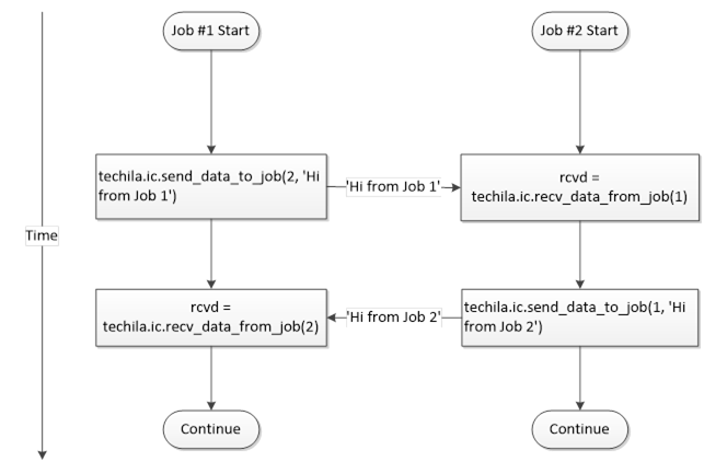
Below is a more detailed explanation on the code sample.
The number of iterations in each Job should be set to one:
.steps=1
The .steps parameter is required for two reasons:
-
Preventing the code from being executed locally on the End-User’s computer (general interconnect requirement)
-
Ensuring that the example will create a Project with two Jobs (example specific requirement)
If the .steps parameter would be removed, the code would be executed locally on the End-User’s computer when estimating the execution time of an iteration. This would generate an error, because the interconnect functions are not defined and cannot be executed on the End-User’s computer.
In this example, the code is also structured so that both iterations must be running simultaneously in different Jobs. For this reason, the value of the .steps parameter has been set to one.
At the start of the code, the interconnect network will be initialized with techila.ic.init(). If no interconnect network can be established, the code will generate an error on this line.
The computational code that is executed on the Techila Workers contain two if-statements, which determine the operations that will be executed in each Job. Job 1 will execute the code inside the first if-statement (i==1) and Job 2 will execute the code inside the other code branch (i==2).
Job 1 will start by executing the send_data_to_job, which is used to transfer data to Job 2. Job 2 respectively starts by executing the ‘recv_data_from_job` function, which is used to read the data, which is being transferred by Job 1.
After Job 2 has received the data, the roles are reversed, meaning Job 2 will transfer data to Job 1.
After Job 1 has received the data from Job 2, both Jobs exit their respective if-statements and execute the wait_for_others() function (line 18), which will act as a synchronization point in the Jobs.
After both Jobs have executed the techila.ic.wait_for_others() function, the techila.ic.disconnect() function will be executed, which will close the connection to the interconnect network.
After the Jobs have been completed, the results will be downloaded and stored to the result variable on the End-User’s computer where the results will be printed on the screen.
6.1.2. Creating the computational Project
To create the computational Project, change your current working directory in your R environment to the directory that contains the example material relevant to this example.
After having browsed to the correct directory, you can source the Local Control Code using command:
source("run_jobtojob.r")
After having sourced the file, create the computational Project using command:
result <- run_jobtojob()
The example screenshot below illustrates the program output, which will display the message strings that were transferred between Jobs.
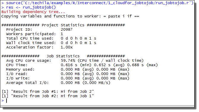
6.2. Broadcasting Data from one Job to all other Jobs
This example is intended to illustrate how to broadcast data from one Job to all other Jobs in the Project. An executable code snippet is provided for the distributed version that uses the cloudfor function.
The material used in this example is located in the following folder in the Techila SDK:
techila\examples\R\Interconnect\2_cloudfor_broadcast
Please note that before you can successfully run this example, your TDCE environment needs to be configured to support Techila interconnect Projects. Please ask your local TDCE Administrator for more information.
Data can be broadcasted from one Job to all other Jobs with the cloudbc function:
bcval = techila.ic.cloudbc(<datatobetransferred>, <sourcejobidx>);
The notation <datatobetransferred> should be replaced with the data you wish to broadcast to other Jobs in the Project. The notation <sourcejobidx> should be replaced with the index of the Job you wish to use for broadcasting the data. The function will return the broadcasted data and it can be stored in a workspace variable; in example syntax shown above it will be stored in the bcval variable.
The figure below illustrates how the techila.ic.cloudbc command could be used to broadcast the value of a local variable x from Job 2 to other Jobs in the Project.
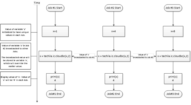
6.2.1. Example code walkthrough
The source code of the example discussed in this Chapter shown below. The commented version of the code can be found in the following file in the Techila SDK:
techila\examples\R\Interconnect\2_cloudfor_broadcast\run_broadcast.r
# Example documentation: http://www.techilatechnologies.com/help/r_interconnect_2_cloudfor_broadcast
run_broadcast <- function() {
# This function contains the cloudfor-loop, which will be used to distribute
# computations to the Techila environment.
#
# During the computational Project, data will be broadcasted from one Job
# to all other Jobs in the Project. The broadcasted data will be returned
# from all Jobs.
#
# Syntax:
#
# source("run_broadcast.r")
# jobres <- run_broadcast()
#

# Copyright Techila Technologies Ltd.

  library(techila)

  # Set loops to three. Will define number of Jobs in the Project.
  loops <- 3

  # Set source Job to two. Will define which Job broadcasts data.
  sourcejob <- 2
  res <- cloudfor (i=1:loops, # Set number of iterations to three.
                      .sdkroot="../../../..", # Location of the Techila SDK 'techila' directory.
                      #.ProjectParameters = list("techila_worker_group" = "IC Group 1"), # Uncomment to use. Limit Project to Workers in Worker Group 'IC Group 1'
                      .steps=1 # Set number of iterations per Job to one.
                      ) %t% {
    # Initialize the interconnect network.
    techila.ic.init()

    # Build message string
    datatotransfer = paste("Hi from Job", i)

    # Broadcast contents of 'datatotransfer' variable from 'sourcejob' to all other Jobs in the Project
    jobres = techila.ic.cloudbc(datatotransfer,sourcejob)

    # Wait until all Jobs have reached this point before continuing
    techila.ic.wait_for_others()

    # Disconnect from the interconnect network
    techila.ic.disconnect()

    # Return the broadcasted data.
    jobres
  }

  # Print and return the results
  for (i in 1:length(res)) {
    print(paste("Result from Job #",i,": ",res[i],sep=""))
  }
  return(res)
}
This example will create a Project with three (3) Jobs. Job 2 will transfer the string Hi from Job 1 to Jobs 1 and 3. The transferred string will be displayed on the End-User’s computer after the Project has been completed.
The value of the sourcejob parameter to two (2), which will be used to define which Job will broadcast the data. If you want to transfer data from another Job, simply change the value to either 1 or 3, depending on which Job you want to use to broadcast the data.
The message that will be broadcasted is a string containing the the Job’s index number. The example table below illustrates values of the datatotransfer variable in each Job, in a Project consisting of 3 Jobs.
Job |
Value of ‘datatotransfer` |
1 |
Hi from Job 1 |
2 |
Hi from Job 2 |
3 |
Hi from Job 3 |
The cloudbc-function that will be used to broadcast the data from one Job to all other Jobs in the Project is shown below.
jobres = techila.ic.cloudbc(datatotransfer,sourcejob)
The value of the variable sourcejob will determine which Job will broadcast data. The data that will be transferred is defined by the value of the datatotransfer variable. With the values used in this example, Job 2 will broadcast the string Hi from Job 2 to all other Jobs in the Project.
In each Job, the techila.ic.cloudbc function will return the string that was broadcasted and store it in the jobres variable.
The line containing techila.ic.wait_for_others() will act as a synchronization point, meaning Jobs will wait until all other Jobs have also executed the function before continuing.
After all Jobs have reached the syncronization point, they will disconnect from the interconnect network.
6.2.2. Creating the computational Project
To create the computational Project, change your current working directory in your R environment to the directory that contains the example material relevant to this example.
After having browsed to the correct directory, you can source the Local Control Code using command:
source("run_broadcast.r")
After having sourced the file, create the computational Project using command:
res <- run_broadcast()
When executed, the code will create a Project consisting of three (3) Jobs. Job 2 will broadcast data to other Jobs in the Project. Below figure illustrates the operations that take place when the code is executed with the syntax shown above.
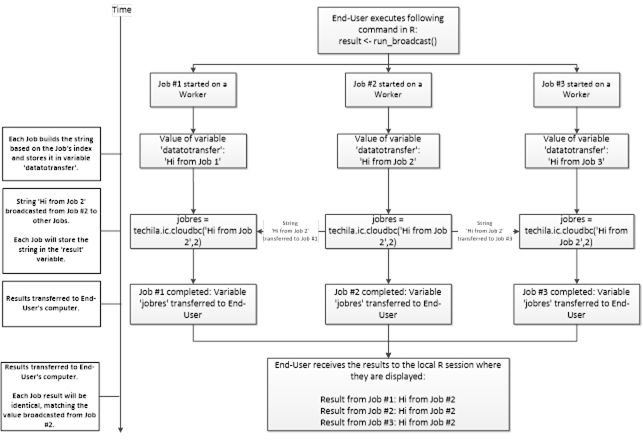
The example screenshot below illustrates the program output, which will display the message string that was broadcasted during the Project.
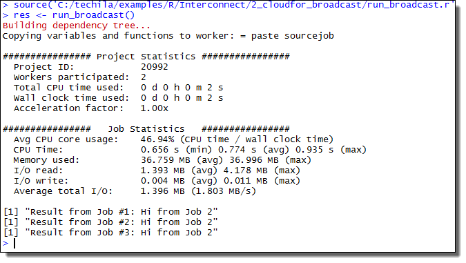
6.3. Transferring Data from all Jobs to all other Jobs
This example is intended to illustrate how to broadcast data from all Jobs to all other Jobs in the Project.
The material used in this example is located in the following folder in the Techila SDK:
techila\examples\R\Interconnect\3_cloudfor_alltoall
Please note that before you can successfully run this example, your TDCE environment needs to be configured to support Techila interconnect Projects. Please ask your local Techila Administrator for more information.
6.3.1. Example code walkthrough
The source code of the example discussed in this Chapter shown below. The commented version of the code can be found in the following file in the Techila SDK:
techila\examples\R\Interconnect\3_cloudfor_alltoall\run_alltoall.r
# Example documentation: http://www.techilatechnologies.com/help/r_interconnect_3_cloudfor_alltoall
run_alltoall <- function() {
# This function contains the cloudfor-loop, which will be used to distribute
# computations to the Techila environment.
#
# This code will create a Project, which will have 4 Jobs. Each Job will send
# a short string to all other Jobs in the Project by using the Techila
# interconnect feature.
#
# Syntax:
#
# source("run_alltoall.r")
# jobres <- run_alltoall()
#

# Copyright Techila Technologies Ltd.

    # Load the techila package
    library(techila)

    # Set loops to four
    loops <- 4
    res <- cloudfor (jobidx=1:loops, # Set number of iterations to four
                      .sdkroot="../../../..", # Location of the Techila SDK 'techila' directory.
                      #.ProjectParameters = list("techila_worker_group" = "IC Group 1"), # Uncomment to use. Limit Project to Workers in Worker Group 'IC Group 1'
                      .steps=1 # Set number of iterations per Job to one.
                     ) %t% {

            # Initialize the interconnect network.
            techila.ic.init()
            dataall = list()

            # Get the number of Jobs in the Project
            jobcount = techila.get_jobcount()

            # Build a simple message string
            msg = paste("Hi from Job", jobidx)

            # For loops for sending data to all other Jobs.
            for (src in 1:jobcount) {
              for (dst in 1:jobcount) {
                if (src == jobidx && dst != jobidx) {
                  techila.ic.send_data_to_job(dst,msg)
                }
                else if (src != jobidx && dst == jobidx) {
                  data = techila.ic.recv_data_from_job(src)
                  dataall = c(dataall, data);
                }
                else {
                  print('Do nothing')
                }
              }
            }
            # Wait until all Jobs have reached this point before continuing
            techila.ic.wait_for_others()

            techila.ic.disconnect()
            dataall
        }

    # Print and return the results
    for (i in 1:length(res)) {
      jobres = unlist(res[i])
      cat("Result from Job #",i,":",jobres, "\n")
    }
    return(res)
}
As can be seend from the example code, data can be transferred to all Jobs from all other Jobs by using the send_data_to_job and recv_data_from_job functions combined with regular for-loops and if-statements. These for-loops and if-statements will need to be implemented so that each Job that is sending data has a matching Job that is receiving data.
The above example code will create a Project with 4 Jobs where simple strings will be transferred from each Job to all other Jobs in the Project.
The number of Jobs in the Project is determined by calling the techila.get_jobcount function, which will return the number of Jobs (4) in the Project.
The message string that will be transferred between Jobs will contain the Job’s index number to indicate which Job sent the message. The table below shows the messages transferred from each Job.
| Job | Message Transferred |
|---|---|
1 |
Hi from Job 1 |
2 |
Hi from Job 2 |
3 |
Hi from Job 3 |
4 |
Hi from Job 4 |
The two for-loops inside the cloudfor-loop contain the code that will decide the order in which Jobs will transfer messages to other Jobs. The transferred messages will be stored to the dataall list, which will be returned to the End-User’s computer.
The interconnect data transfers that take place during the Project are illustrated in the figure below. The arrows indicate that interconnect data is being transferred. The values in parentheses correspond to the values of the src and dst loop counters. For example, arrow with value (1,3) means that Job 1 is sending the msg string to Job 3. If src is equal to dst (e.g. (2,2)), no data is transferred because the source and target are the same.
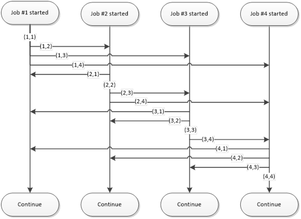
6.3.2. Creating the computational Project
To create the computational Project, change your current working directory in your R environment to the directory that contains the example material relevant to this example.
After having browsed to the correct directory, you can source the Local Control Code using command:
source("run_alltoall.r")
After having sourced the file, create the computational Project using command:
res <- run_alltoall()
When the command is executed, the code will create a Project consisting of four (4) Jobs. Each Job will transfer a simple string to all other Jobs in the Project. These transferred strings will then be returned and displayed on the End-User’s computer as illustrated in the screenshot below.
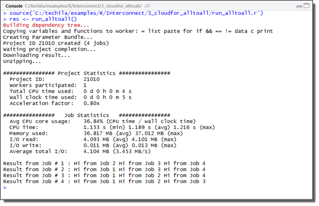
6.4. Executing a Function by Using CloudOp
This example is intended to illustrate how to execute a function by using the cloudop-function.
The material used in this example is located in the following folder in the Techila SDK:
techila\examples\R\Interconnect\4_cloudfor_cloudop
Please note that before you can successfully run this example, your TDCE environment needs to be configured to support Techila interconnect Projects. Please ask your local Techila Administrator for more information.
The cloudop-function executes the given operation across all the Jobs and returns the result to all Jobs, or the target Job:
result = techila.ic.cloudop(<op>, <data>, <target>)
The effect of the input arguments is explained below.
The <op> notation should be replaced with the function you wish to execute across all Jobs. For example the following syntax could be used to execute the R max function.
result = techila.ic.cloudop(max, <data>, <target>)
It is also possible to execute custom, user defined functions with cloudop. For example, if you have developed a custom function called multiply, then you could execute this with the following syntax.
result = techila.ic.cloudop(multiply, <data>, <target>)
The <data> notation should be replaced with the input data you wish to pass to the function defined in <op> as an input argument.
The <target> is an optional argument, which can be used to define how the final result of the operation will be returned. When the <target> argument is omitted or set to zero, cloudop will return the final result in all Jobs.
The <target> argument can also be used to transfer the final result to a specific Job. For example, if the value of the <target> argument is set to one (1), the result of the <op> will only be returned in Job 1. In all other Jobs, the cloudop function would return the value NULL.
Functions executed with cloudop will need to meet following requirements:
-
The function must accept two input arguments
-
The function must return one output value. The format of this output value must be such that it can be given as an input argument to the custom function. This is because the operations will be executed using a binary tree structure, which means that the output of the custom function will be also used as input for the function when function is called later in the tree structure.
The example code snippet below shows custom function called multiply, which meets the above requirements.
multiply <- function(a, b) {
    return(a *b)
}
Example 1: In the example code snippet below, the min function is used to find the minimum value of local workspace variables (variable x). The minimum value will then be transferred to Job 2, where it will be stored in the xmin variable. All other Jobs will return the value NULL as the result.
run_cloudop <- function() {
  library(techila)
  inputdata <- c(10,5,20)
  loops <- length(inputdata)
  results <-  cloudfor (i=1:loops,
                        .steps=1
  ) %t% {
    techila.ic.init()
    x <- inputdata[i]
    xmin <- techila.ic.cloudop(min, x, 2)
    techila.ic.disconnect()
    xmin
  }
  print(results)
}
The operations that take place on the Techila Workers when the above code snippet is executed are illustrated in the figure below.
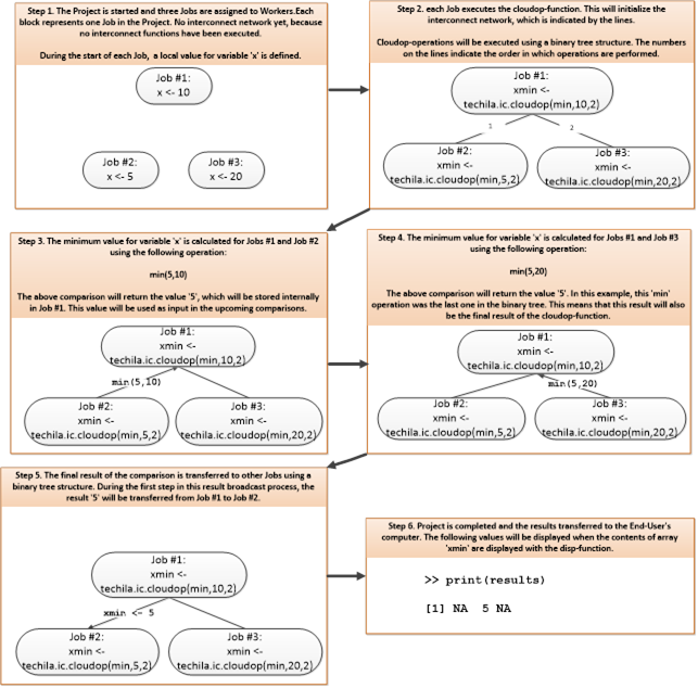
Example 2: In the example code snippet below, the min function is used to find the global minimum value of local workspace variables (variable x). The minimum value will then be broadcasted to all Jobs and stored in an array. The code snippet would create a Project containing nthree (3) Jobs.
run_cloudop <- function() {
  library(techila)
  inputdata <- c(10,5,20)
  loops <- length(inputdata)
  results <-  cloudfor (i=1:loops,
                        .steps=1
  ) %t% {
    techila.ic.init()
    x <- inputdata[i]
    xmin <- techila.ic.cloudop(min, x)
    techila.ic.disconnect()
    xmin
  }
  print(results)
}
The operations that take place on the Techila Workers when the above code snippet is executed are illustrated in the figure below.
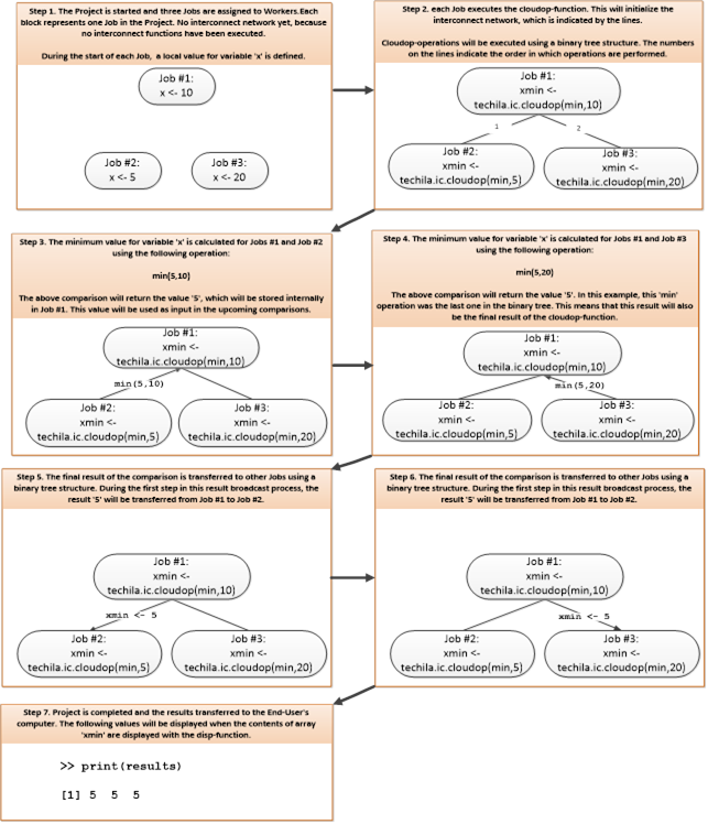
Summing values with cloudsum
The cloudsum function can be used to sum the defined variables. The operating principle of this function is similar to cloudop, with the exception that the cloudsum function can only be used to perform summation. The general syntax of the function is shown below.
result = techila.ic.cloudsum(<data>,<target>)
The <data> notation defines the input data that will be summed together.
The <target> can be used to define how the final result of the operation will be returned. When the <target> argument is omitted or set to zero, cloudsum will return the final result in all Jobs.
The <target> argument can also be used to transfer the final result to a specific Job. For example, if the value of the <target> argument is set to one (1), the summation result will only be returned in Job 1. In this case, the cloudsum function will return the value NULL in all other Jobs.
Example:
The code snippet below could be used to create a Project with three Jobs. Each Job executes the cloudsum to sum randomly generated numbers. The summation result would be returned in all Jobs and would be stored in the variable sumval.
run_cloudop <- function() {
  library(techila)
  loops <- 3
  results <-  cloudfor (i=1:loops,
                        .steps=1
  ) %t% {
    techila.ic.init()
    sumval <- techila.ic.cloudsum(runif(1))
    techila.ic.disconnect()
    sumval
  }
  print(results)
}
6.4.1. Example code walkthrough
The source code of the example discussed in this Chapter shown below. The commented version of the code can be found in the following file in the Techila SDK:
techila\examples\R\Interconnect\4_cloudfor_cloudop\run_cloudop.r
# Example documentation: http://www.techilatechnologies.com/help/r_interconnect_4_cloudfor_cloudop
run_cloudop <- function() {
# This function contains the cloudfor-loop, which will be used to distribute
# computations to the Techila environment.
#
# This code will create a Project, which will have 4 Jobs. Each Job will
# start by generating a random number locally. The 'cloudop' function will
# then be used to find the minimum value from these local variables.
# To create the Project, use command:
#
# Syntax:
#
# source("run_cloudop.r")
# jobres <- run_cloudop()
#

# Copyright Techila Technologies Ltd.

  # Load the techila package
  library(techila)
  loops <- 3
  results <-  cloudfor (i=1:loops,
                        .sdkroot="../../../..", # Location of the Techila SDK 'techila' directory.
                        #.ProjectParameters = list("techila_worker_group" = "IC Group 1"), # Uncomment to use. Limit Project to Workers in Worker Group 'IC Group 1'
                        .steps=1 # Set number of iterations per Job to one.
                        ) %t% {

    # Initialize the interconnect network.
    techila.ic.init()

    # Set the random number generator seed
    set.seed(i)

    # Generate a random number
    data=runif(1)

    # Execute the 'multiply' function with input 'data' across all Jobs.
    # The result of the multiplication operation will be stored in 'mulval' in all Jobs.
    mulval <- techila.ic.cloudop(multiply,data)

    # Wait until all Jobs have reached this point before continuing
    techila.ic.wait_for_others()

    # Disconnect from the interconnect network
    techila.ic.disconnect()

    # Return the multiplication value as the result
    mulval
  }

  # Print and return the results.
  for (i in 1:length(results)) {
    jobres = unlist(results[i])
    cat("Result from Job #",i,":",jobres, "\n")
  }
}

# Define a simple function which performs multiplication.
# This function will be executed across all Jobs by using the 'techila.ic.cloudop' function.
multiply <- function(a,b) {
  return(a * b)
}
This example will create a Project with three (3) Jobs. Each Job will generate a random number, which will be multiplied by using the cloudop function. The multiplication result will be displayed on the End-User’s computer after the Project has been completed.
Each Job will set the random number generator seed at the start of the Job, which ensures that random numbers can be generated repeatedly.
After setting the seed, each Job generates one random number and stores the value in the data variable.
The multiply function is then executed across all Jobs with the input values stored in the data variable. The syntax used in this example defines two input arguments to the cloudop function (<op>, <data>), meaning the third input argument (<target>) has not been defined. This means that the final result of the cloudop function will be stored in variable mulval in all Jobs.
The definition for the multiply function is located at the end of the code. This function accepts two input arguments, multiplies them and returns the multiplication value as the result. This means that the multiply function meets the requirements for functions that can be executed with cloudop.
6.4.2. Creating the computational Project
To create the computational Project, change your current working directory in your R environment to the directory that contains the example material relevant to this example.
After having browsed to the correct directory, you can source the Local Control Code using command:
source("run_cloudop.r")
After having sourced the file, create the computational Project using command:
res <- run_cloudop()
The example screenshot below illustrates the program output, which will display the value of the multiplication result calculated during the Project. Each Job will return the same value, because the syntax of the cloudop-function used in this example did not define the <target> argument.
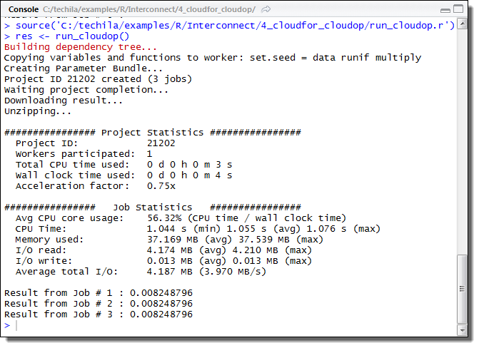
7. Cloud Control
The Techila cloud control feature allows controlling Techila Worker instances in various clouds.
This Chapter contains walkthrough of a simple example, which illustrates how to use the Techila cloud control functions. The example is the same as the first example in the peach tutorial with the cloud control functions added.
The material discussed in this example is located in the following folder in the Techila SDK:
techila\examples\R\Features\cloud_control
7.1. Distributed version of the program
All arithmetic operations in the locally executable function are performed in the for loop. There are no recursive data dependencies between iterations, meaning that the all the iterations can be performed simultaneously. This is done by placing the computational instructions in the Techila Worker Code (distribution_dist.r).
Local Control Code in the R script run_cloudcontrol.r is used to start Techila Worker cloud instances, set the idle shutdown time for the instances, create the computational Project and terminate the instances in the end. The Techila Worker Code in the distribution_dist.r file is transferred to the Techila Workers where script will automatically be sourced at the preliminary stages of the Job. After the R script has been sourced, the function distribution_dist will be executed.
7.2. Local Control Code
The Local Control Code used to control the cloud Worker instances and create the computational Project is shown below.
# Example documentation: https://docs.techilatechnologies.com/help/techila-distributed-computing-engine/r-techila-distributed-computing-engine.html#_cloud_control
# Copyright Techila Technologies Ltd.

# This function contains the Local Control Code, which will start a cloud worker
# instance, create a computational Project and terminate the cloud worker instance.
#
# Usage:
# source("run_cloudcontrol.r")
# result <- run_cloudcontrol(jobs)
# jobs: the number of Jobs in the Project
#
# Example:
# result <- run_cloudcontrol(5)
run_cloudcontrol <- function(jobs) {

  # Load the techila library
  library(techila)

  # Initialize connection to the Techila Server
  init()

  # Start 1 worker instance with 4 cores (default instance type)
  techila:::deploy_workers(1)

  # To specify instance type and start 4 instances, use command:
  #   techila:::deploy_workers(4, "<machinetype>");
  # where available values for <machinetype> depend on the cloud. The default instance types are
  # Google: n1-standard-4
  # AWS:    c5.large
  # Azure:  Standard_D2s_v3

  # Set worker instances idle shutdown delay to 1 minute
  techila:::set_auto_delete_delay(1)

  # Create the computational Project with the peach function.
  result <- peach(funcname = "distribution_dist",    # Function that will be called on Workers
                  files = list("distribution_dist.r"), # R-file that will be sourced on Workers
                  peachvector = 1:jobs,                 # Number of Jobs in the Project
                  sdkroot = "../../../..")              # Location of the techila_settings.ini file

  # Shutdown instances
  techila:::shutdown_workers()

  # Uninitialize the connection
  uninit()

  # Display results after the Project has been completed. Each element
  # will correspond to a result from a different Job.
  print(as.numeric(result))
  result
}
The script defines one function called run_cloudcontrol, which requires one input parameter. This input parameter will be used to specify the number of Jobs into which the Project should be split. This will be further done by using the jobs input parameter, which defines the length of the peachvector.
In this example, no input arguments are required by the function that will be executed on the Techila Workers. This means that the params parameter does not need to be defined.
Techila Server connection is initialized by calling init. After this, deploy_workers is used to start Techila Worker cloud instances. In this case, one Worker instance with the default configuration is started.
Additionally, idle shutdown delay is set by calling set_auto_delete_delay. This makes the cloud instance(s) to be automatically terminated when they have been idling (no computational projects are running) for the configured period. In this case, the delay is set to one minute.
To terminate the Techila Worker cloud instances, shutdown_workers is called. Without this, the instances would also be terminated automatically after the configured idle shutdown delay.
The internal state of Techila connection and related resources are cleaned by calling uninit.
At the final stages of the code, as soon as the results have been transferred back to the End-User’s local computer, the results will be converted to numeric format.
7.3. Techila Worker Code
The Techila Worker Code that performs the computations is shown below.
# Example documentation: http://www.techilatechnologies.com/help/r_tutorial_1_distribution
# Copyright Techila Technologies Ltd.

# This function contains the function that will be executed during
# computational Jobs. Each Job will perfom the same computational
# operations: calculating 1+1.
distribution_dist <- function() {

  # Store the sum of 1 + 1 to variable 'result'
  result <- 1 + 1

  # Return the value of the 'result' variable. This value will be
  # returned from each Job and the values be displayed on the
  # End-Users computer after the Project is completed.
  return(result)
}
7.4. Creating the computational Project
To create the computational Project, please change your current working directory in your R environment to the directory containing the example material for this example.
After having browsed to the correct directory, you can source the Local Control Code using command:
source("run_cloudcontrol.r")
After having sourced the R script, execute the function using command:
result <- run_cloudcontrol(3)
This will create a computational Project consisting of three Jobs. Each of the Jobs will be extremely short, as each Job consists of simply summing up two integers; 1+1.
8. Appendix
8.1. Appendix 1: Peach Parameters with Example Values
| Parameter | example | Description |
|---|---|---|
callback |
callback="function_1" |
Calls given function for each result and returns callback function’s result as the |
close |
close=FALSE |
Closes the handle. Affects what is returned from peach, see Appendix 2 for details. Default value: TRUE |
databundles |
databundles = list(list(datafiles = list("file1","file2")) |
Used to create Data Bundles. Listed files will be included in the Data Bundle(s). |
datafiles |
datafiles=list("datafile.txt") |
Determines which files will be stored in the Parameter Bundle and transferred with each Job. In this example, a file called datafile.txt will be transferred. |
donotuninit |
donotuninit =TRUE |
Does not uninitialize the TDCE environment. Affects what is returned from peach, see Appendix 2 for details. Default value: FALSE |
donotwait |
donotwait = TRUE |
Returns immediately after the Project has been created. Affects what is returned from peach, see Appendix 2 for details. Default value: FALSE |
filehandler |
filehandler="function_2" |
Calls given file handler function for each additional result file. |
files |
Case 1: files=list("temp_dist.r") Case 2: files=list("C:/temp/temp2_dist.r") |
Names of the R scripts that will be sourced at the preliminary stages of a computation Job. Case 1: The "temp_dist.r" file is included from the current working directory Case 2: The "temp_dist2.r" file is included from the directory "C:/temp/" |
funcname |
Case 1: funcname="function_1" Case 2: funcname=func_handle |
Name of the function that will be called in the computational Job. Case 1: "function_1" refers to a function defined in an R script listed in the files parameter. Case 2: func_handle refers to a function defined in the workspace |
sdkroot |
sdkroot="C:/techila" |
Determines the path of the |
imports |
imports="example.bundle.v1,example.bundle2.v1" |
Determines additional Bundles that will be imported in the Project. In the example, Bundles exporting |
initFile |
initFile="C:/ex/techila_settings.ini" |
Specifies the path of the Techila config file (techila_settings.ini). |
jobinputfiles |
jobinputfiles = list(datafiles = list("file1_job1","file1_job2"), filenames = list("workername") ) |
Assigns Job-Specific input files that will be transferred with each computational Job. |
messages |
messages=FALSE |
Determines if messages will be displayed regarding Project statistics and other Project related information.Default value: TRUE |
outputfiles |
outputfiles=list("file1","file2") |
Speficies additional output files that will be transferred to the End-User’s computer from Techila Workers. |
params |
params =list(a=2,b="john","<param>") |
A list of parameters that will be used as input arguments by the executable function. |
peachvector |
peachvector=4:1 |
The "<param>" parameter is replaced by elements of the peachvector. In this example, elements of the peachvector are 4,3,2,1. The length of the peachvector also determines the number of Jobs in the Project. |
priority |
Case 1: priority="high" Case 2: priority=2 |
Determines the priority of the Project. Adjusting the priority value can be used to manage the order in which computational Projects created by you are processed. Projects with priority= 1 receive the most resources and Projects with priority=7 the least amount of resources. Default value: 4 |
projectid |
projectid = 1234 |
Determines the Project ID number of the Project to which the |
removeproject |
removeproject=FALSE |
Determines if Project related data will be removed from the Techila Server after the Project is completed.Default value: TRUE |
RVersion |
RVersion="2120" |
Specifies which R Runtime Bundle is required to execute the computational Jobs. If the RVersion parameter is not specified, the version of the R environment used to create the Project will be used. |
snapshot |
snapshot = TRUE |
Enables snapshotting in the Project with the default snapshot file name and snapshot transfer interval. Default value: FALSE |
snapshotfiles |
snapshotfiles = "test.txt" |
Specifies the name of the snapshot file. If specified, this value overrides the default value. Default value: "snapshot.rda" |
snapshotinterval |
snapshotinterval=30 |
Specifies a snapshot transfer interval in minutes. If specified, this value overrides the default snapshot transfer interval.Default value: 15 |
stream |
stream = TRUE |
Enables Job results to be streamed immediately after they have been transferred to the Techila Server. In this example, streaming is enabled. Default value: FALSE |
ProjectParameters |
Case 1:ProjectParameters = list("techila_client_memorymin" = "1073741824", "techila_client_os" = "Windows") |
Defines additional Project parameters. Case 1: Defines that only Techila Workers with a Windows operating system and 1 GB of free memory can be assigned Jobs. |
BundleParameters |
Case 1: BundleParameters=list("ExpirationPeriod" = "2 h") |
Defines parameters for the Parameter Bundle.Case 1: Defines that the Parameter Bundle should be stored for 2 hours on Techila Workers. |
BinaryBundleParameters |
Case 1: BinaryBundleParameters=list("ExpirationPeriod" = "2 h") |
Defines parameters for the Executor Bundle. Case 1: Defines that the Executor Bundle should be stored for 2 hours on Techila Workers. |
8.2. Appendix 2: Peach Return Values
The table below contains a description on what the peach function will return, depending on the values of the donotuninit, donotwait and close parameters.
| donotuninit | donotwait | close | peach return value | Note |
|---|---|---|---|---|
False |
False |
True |
Result |
This is default combination. |
False |
True |
True |
Project ID |
- |
True |
False |
True |
Result |
This combination should be used in iterative Projects. |
True |
True |
False |
Handle |
- |
True |
True |
True |
Project ID |
- |