1. Introduction
This example illustrates how to use Techila Distributed Computing Engine to speed up Value-at-Risk computations implemented with Python and follows the same approach discussed in the paper below.
Please note that the Python version of this example was created after the original publication of the paper discussed below, meaning that the paper does not include the performance statistics for the Python version of the code.
If you are unfamiliar with the TDCE terminology or are interested in more general information about TDCE, please see Introduction to Techila Distributed Computing Engine. More details about the TDCE Python application program interface (API) can be found in Techila Distributed Computing Engine with Python.
2. Code Overview
One of the most common risk measures in the finance industry is Value-at-Risk (VaR). Value-at-Risk measures the amount of potential loss that could happen in a portfolio of investments over a given time period with a certain confidence interval. It is possible to calculate VaR in many different ways, each with their own pros and cons. Monte Carlo simulation is a popular method and is used in this example.
In the simplified VaR model used in the example, the value of a portfolio of financial instruments is simulated under a set of economic scenarios. The set of financial instruments in this example is limited to a set of fixed coupon bonds and equity options. The scenarios can be analyzed independently, meaning that the computations can be sped up significantly by analyzing the scenarios simultaneously on a large number of Techila Worker nodes.
This example is available for download at the following link:
The contents of the zip file is shown below for reference:
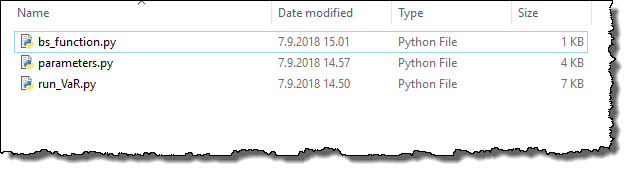
The run_VaR.py file is main file used in this example and contains the definition for function run_demo, which is the function used to run the example. Depending on the value of the input argument given to the run_demo function, it can be used to run the VaR computations either locally (run_demo(local=True)) or in TDCE (run_demo(local=False)).
2.1. Data Locations & Management
This example uses a set financial instruments, which are generated when the parameters.py file is executed locally. This file is included in the zip-file, as can be seen from the previous screenshot.
When the parameters.py file is executed, variables will be defined in the local Python workspace. The data stored in these variables will be used when analyzing the scenarios.
When analyzing the scenarios locally, the values of variables needed in the computations will be passed to the computationally intensive function as input arguments, as in any other standard Python application.
In the distributed version of this application, variables will be transferred to Techila Workers participating in the computations by using the peach function’s params parameter.
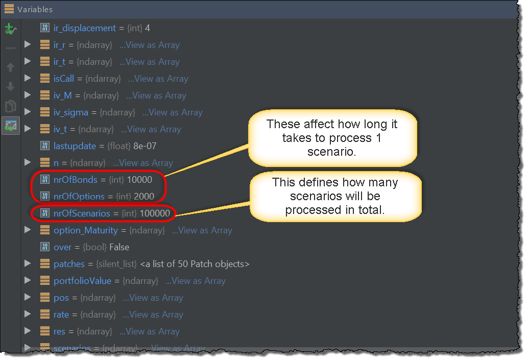
The screenshot below illustrates which variables will be created by the parameters.py file. Parameters nrOfOptions and nrOfBonds will determine the number of financial instruments in the portfolio and will affect how long does it take to process one scenario (more instruments means more processing time required per scenario.). Parameter nrOfScenarios determines the number of scenarios that will be processed in total. In the local version, the nrOfScenarios determines the number of iterations in the for loop structure and in the distributed version, this will be used to calculate how many Jobs will be used to process the computations.
2.2. Sequential Local Processing
The computations can be executed locally by with the following syntax:
| Syntax for Python 2 | Syntax for Python 3 |
|---|---|
|
|
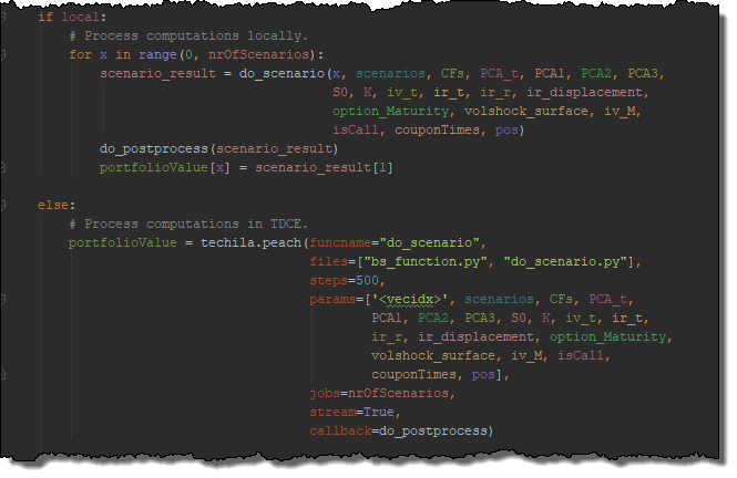
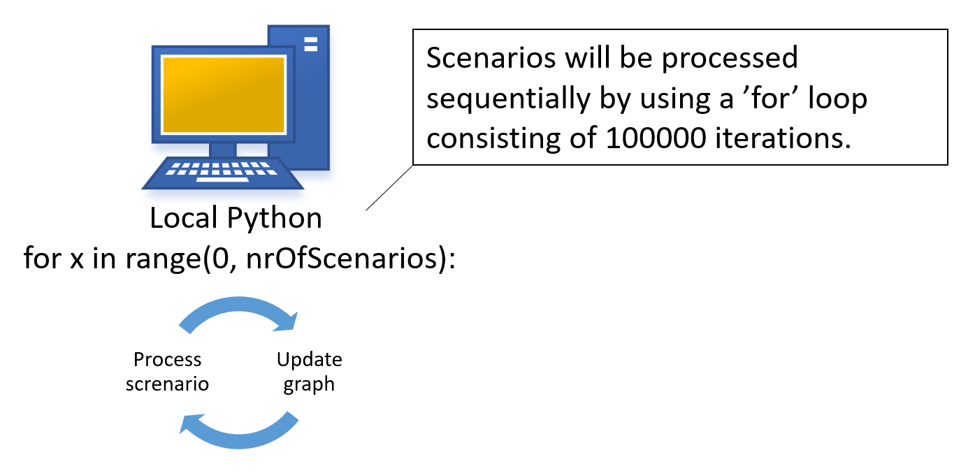
When executed locally, the computations will be processed using the for loop shown below.
# Process computations locally.
for x in range(0, nrOfScenarios):
    scenario_result = do_scenario(x, scenarios, CFs, PCA_t, PCA1, PCA2, PCA3,
                                  S0, K, iv_t, ir_t, ir_r, ir_displacement,
                                  option_Maturity, volshock_surface, iv_M,
                                  isCall, couponTimes, pos)
    do_postprocess(scenario_result)
    portfolioValue[x] = scenario_result[1]
Each iteration processes one scenario and stores the computational result in portfolioValue. Each iteration is also independent, meaning there are no recursive dependencies. The results are visualized by performing a do_postprocess call, which updates the histogram figure with new scenario data at 3 second intervals.
2.3. Distributed Processing
The computations can be executed in Techila Distributed Computing Engine by using the following Python syntax:
| Syntax for Python 2 | Syntax for Python 3 |
|---|---|
|
|
This will result in the following code being executed, which will create the computational Project.
# Process computations in TDCE.
portfolioValue = techila.peach(funcname="do_scenario",
                               steps=500,
                               files=["bs_function.py","do_scenario.py"],
                               params=['<vecidx>', scenarios, CFs, PCA_t,
                                        PCA1, PCA2, PCA3, S0, K, iv_t, ir_t,
                                        ir_r, ir_displacement, option_Maturity,
                                        volshock_surface, iv_M, isCall,
                                        couponTimes, pos],
                               jobs=nrOfScenarios,
                               stream=True,
                               callback=do_postprocess)
The peach syntax parameters are explained below:
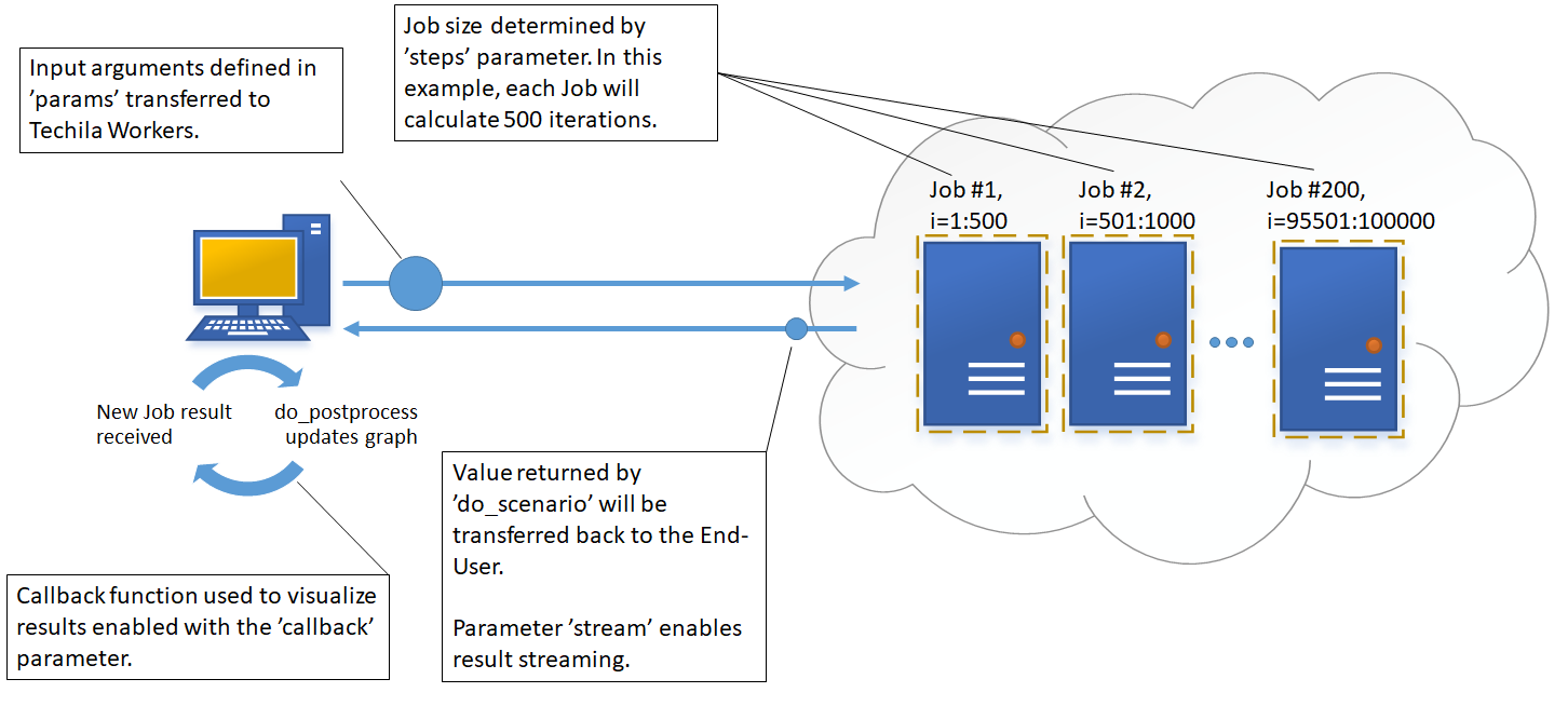
The funcname parameter defines that each Job will execute the do_scenario function. With the defaulta parameters used in this example, one execution of the do_scenario is quite quick (approximately 0.1 seconds) and would result in poor efficiency in the Job due to overheads related to data transfers and initializations. We can greatly improve the efficiency by using the steps parameter to increase the number of times the function is executed in the Job, thus increasing the amount of meaningful computational work per Job. In this example, steps has been set to 500, meaning each Job will execute the do_scenario function for 500 times. This means that each Job will process 500 scenarios and will return a list containing the scenario results.
The files parameter is used list which files be transferred to the Techila Workers. In this example, we will need access to files bs_function.py and do_scenario.py files, which contain function definitions for the functions used in the computations. The TDCE system will automatically make functions defined in the files available in the base workspace used in the Job.
The input arguments needed by the do_scenario function have been defined by using the params parameter, where '<vecidx>' will be used to index the list containing the scenarios. These are identical as in the locally executable version with the exception that the value of the for loop counter has been replaced with the '<vecidx>'. This keyword is recognized by the TDCE system and will automatically be replaced by the Jobidx value, which will be unique in each Job. For example, in Job #1 the value will be 0, in Job #2 it will be 1 and so forth.
The total number of Jobs in the Project is defined by dividing the value of the jobs parameter (total number of scenarios) with the value of the steps parameter (scenarios processed in each Job). For example, if nrOfScenarios=100000, then the Project would contain 200 Jobs (100000 / 500 = 200). In situations where the steps parameter is not used, the number of Jobs set to match the value of the jobs parameter.
The stream parameter has been set to True, which means results will be streamed from the Techila Server to the End-User’s computer as soon as they are available. All Job results will be postprocessed by the do_postprocess function, which will visualize results using a histogram graph.
3. Performance Comparison
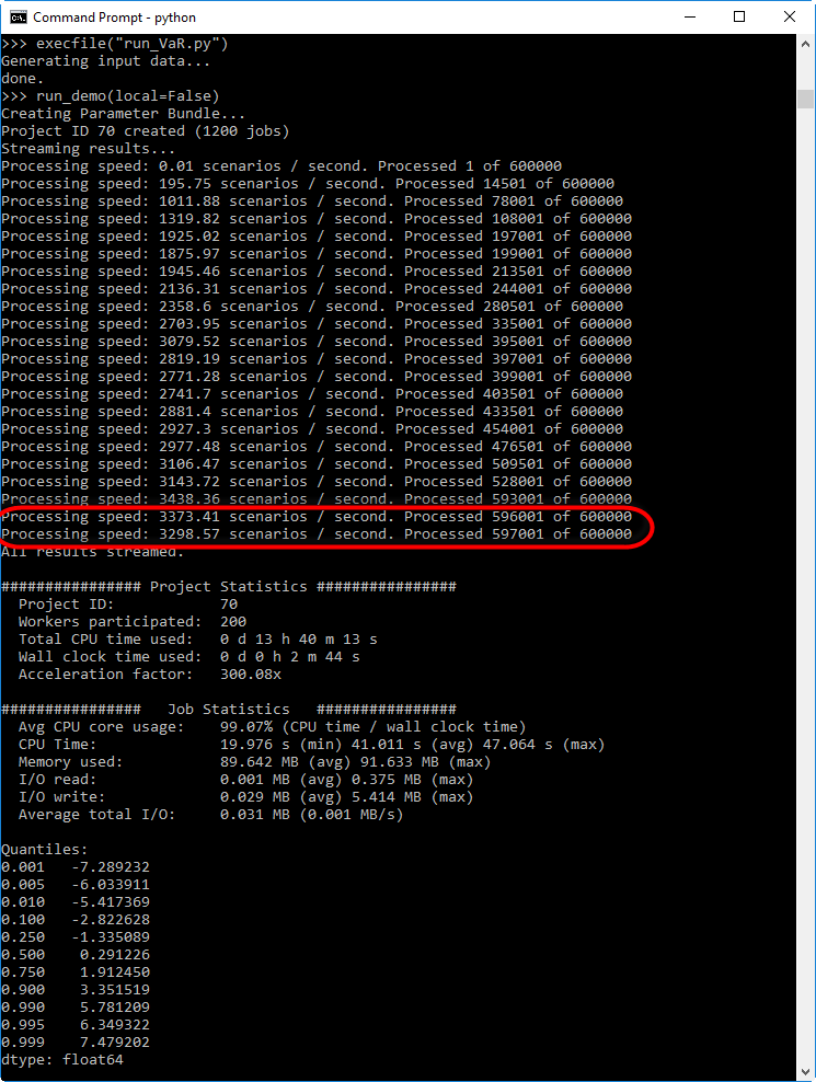
When the run_demo function is executed, the callback function (do_postprocess) will print information about how quickly scenarios are being processed on average. This information can be used to compare the performance of the local version and the distributed version of code.
The average processing speed is calculated using the following formula:
\(Average Processing Speed = {Scenarios Processed \over Elapsed Time} \)
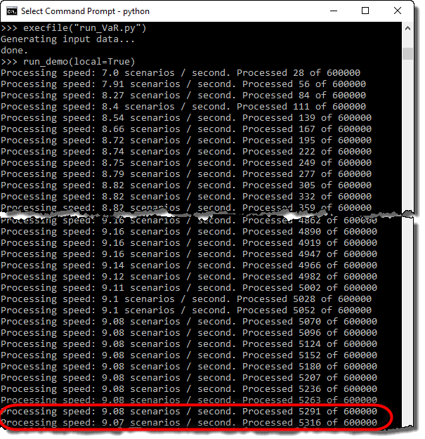
The value of ElapsedTime seen in the formula is measured from the start of the run_demo function. Respectively the callback function do_postprocess will be used to calculate the elapsed time since the program was started and how many scenarios have been processed so far. This information will then be used to display the average processing speed each time the histogram graph is updated. Please note that because the timer starts as soon as the do_postprocess function is started, there will be a short period at the start of the computations where the processing speed will be lower. As more and more scenarios are processed, the average processing speed displayed will become more representative of the actual processing speed.
The processing speed of the local version will mostly depend on the CPU characteristics of the computer you are using to run the code. The screenshot below illustrates the processing speed when running the computations on a Intel i5-5200U CPU @ 2.20 GHz.
The processing speed of the distributed version will mostly depend on the number of Techila Worker CPU cores available for computations. The screenshot below illustrates the processing speed when using 400 Techila Worker CPU cores.