1. MATLAB - Option Pricing Model Calibration
This example illustrates how to use Techila Distributed Computing Engine to speed up the calibration of an option pricing model implemented with MATLAB.
The information on this page is intended to supplement the information in the original paper discussing this application. You can download the paper using the link shown below:
1.1. Introduction
Financial institutions can be exposed to the dynamics of hundreds of securities via derivative contracts, which requires robust hedging strategies with well-calibrated volatility models. The calibration of these models can take a long time, especially if state-of-the-art non-affine volatility models are used.
In a situation where there are several underlying assets for which a model(s) should be calibrated, the computations can be accelerated by using Techila Distributed Computing Engine.
This example is available for download at the following link:
The contents of the zip file is shown below for reference:
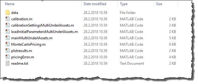
1.2. Data Locations & Management
This example uses a set of pre-generated data files, which are located in the data directory. File priceDataMultiAssets.mat contains a set of assets used in the calibration process and file initialParameterSettings.mat contains the initial parameters for the computations.
The contents of these files are loaded to the local MATLAB workspace, which creates variables named data and initialParameterSettings.
The screenshot below shows what the variables look like in the MATLAB workspace.
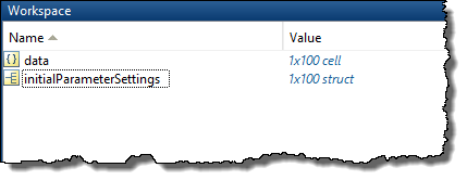
The data stored in variables data and initialParameterSettings will be used when calibrating the model. These variables contain data for 100 assets.
When calibrating the model locally, the values of variables needed in the computations will be accessed from the local workspace, as in any other standard MATLAB application.
In the distributed version of this application, variables will be automatically transferred to Techila Workers participating in the computations, meaning they will also be accessible during the Jobs.
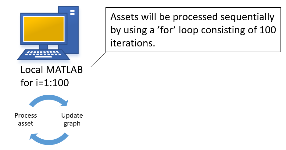
1.3. Sequential Local Processing
The computations could be executed locally by using a for loop structure shown below. Please note that the code package does not include a locally executable version, but the cloudfor version can be easily modified into a local for version as shown in the code snippet below.
for i = 1:settings.numberOfAssets
% ith volatility surface data
rng(i) % Fixed seed for repeatability
% ith volatility surface data
data_i = data{i};
% Initial parameters
parametersInitial = initialParameterSettings(i);
% Calibration
[parametersFinal, fFinal(i, 1), fInitial(i, 1), exitFlag(i, 1)] = ...
calibration(data_i, settings, parametersInitial, i);
% Store the results
results{i}.kappaInitial = parametersInitial.kappa;
results{i}.kappaFinal = parametersFinal.kappa;
results{i}.thetaInitial = parametersInitial.theta;
results{i}.thetaFinal = parametersFinal.theta;
results{i}.xiInitial = parametersInitial.xi;
results{i}.xiFinal= parametersFinal.xi;
results{i}.rhoInitial = parametersInitial.rho;
results{i}.rhoFinal = parametersFinal.rho;
results{i}.gammaInitial = parametersInitial.gamma;
results{i}.gammaFinal = parametersFinal.gamma;
results{i}.V0Initial = parametersInitial.V0;
results{i}.V0Final = parametersFinal.V0;
disp([num2str(i),'th calibration finished with value ', num2str(fFinal(i, 1))]);
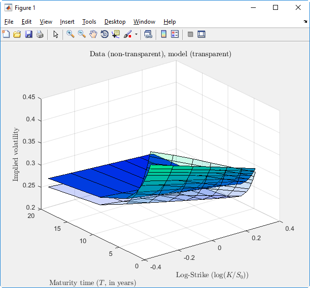
endEach iteration stores the computational result in the results. Each iteration is independent, meaning there are no recursive dependencies. A graph for each model will be generated sequentially as the model is calibrated. The graphs are generated by the commands used in the pricingError function.
The screen capture below shows one the generated model surfaces.
1.4. Distributed Processing
The code below shows the cloudfor version of the code, which will perform the computations in Techila Distributed Computing Engine. The syntax shown below will essentially push all code between the cloudfor and cloudend keywords to Techila Distributed Computing Engine where it will be executed on Techila Workers.
In this example, the result data will be visualized using two different graphs:
-
A summary graph displaying the errors for each individual asset.
-
A model surface for the first asset (Job #1).
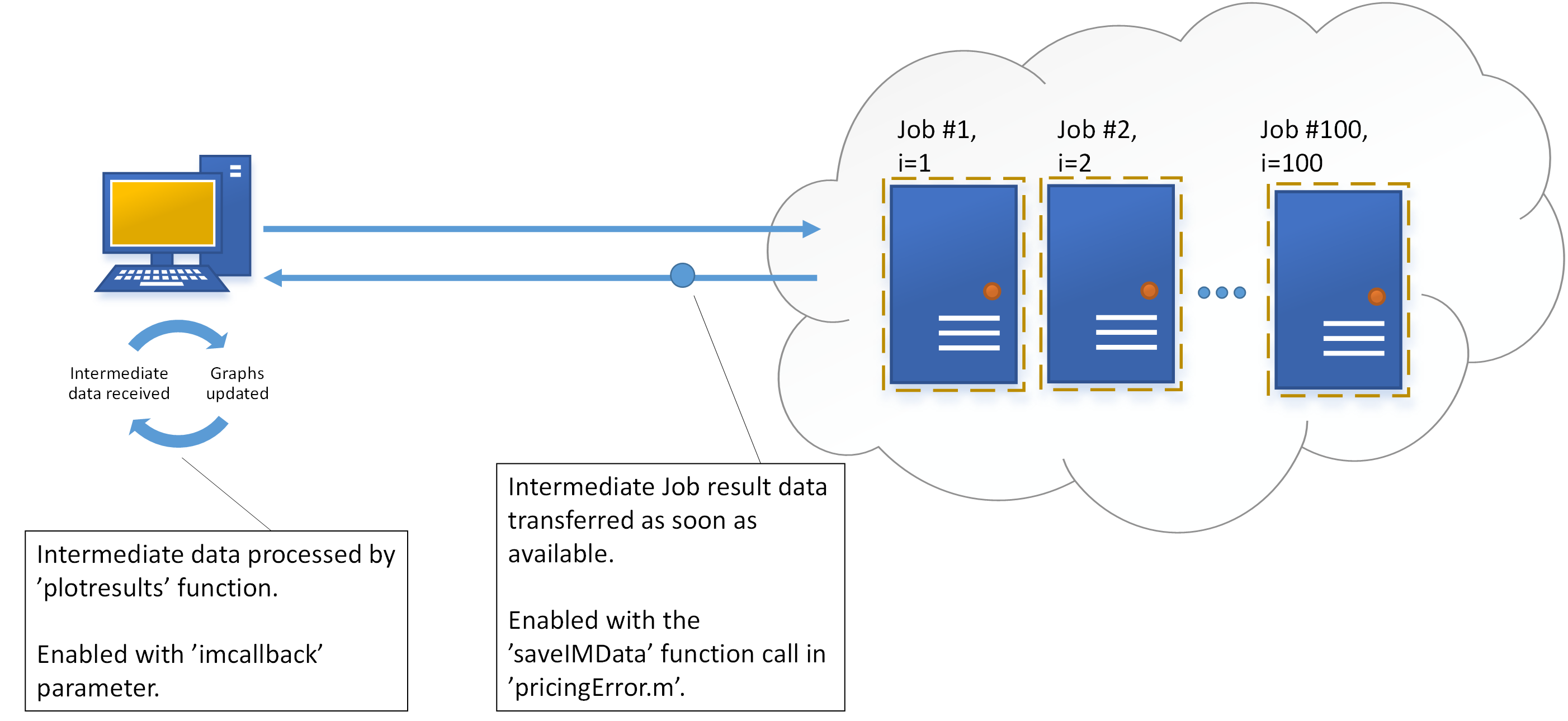
The data used to generate the graphs is transferred by using a Techila Distributed Computing Engine feature called Intermediate Data, which allows transferring and processing of workspace variables generated in the Jobs, while the Jobs are running. This means that Intermediate Data can be used to get immediate feedback from the computational processes, allowing responsive result data visualization and troubleshooting.
Generally speaking, all parameters that start with %cloudfor are optional control parameter used to fine tune the behaviour of the computations. The effect of the control parameters is illustrated in the image below. For more information about the cloudfor helper function, please see Techila Distributed Computing Engine with MATLAB.
More information about the used control parameters and features can also be found in the source code comments.
cloudfor i = 1:settings.numberOfAssets
%cloudfor('imcallback','plotresults(TECHILA_FOR_IMRESULT,h)')
% ith volatility surface data
if isdeployed
rng(i) % Fixed seed for repeatability
% ith volatility surface data
data_i = data{i};
% Initial parameters
parametersInitial = initialParameterSettings(i);
% Calibration
[parametersFinal, fFinal(i, 1), fInitial(i, 1), exitFlag(i, 1)] = ...
calibration(data_i, settings, parametersInitial, i);
% Store the results
results{i}.kappaInitial = parametersInitial.kappa;
results{i}.kappaFinal = parametersFinal.kappa;
results{i}.thetaInitial = parametersInitial.theta;
results{i}.thetaFinal = parametersFinal.theta;
results{i}.xiInitial = parametersInitial.xi;
results{i}.xiFinal= parametersFinal.xi;
results{i}.rhoInitial = parametersInitial.rho;
results{i}.rhoFinal = parametersFinal.rho;
results{i}.gammaInitial = parametersInitial.gamma;
results{i}.gammaFinal = parametersFinal.gamma;
results{i}.V0Initial = parametersInitial.V0;
results{i}.V0Final = parametersFinal.V0;
disp([num2str(i),'th calibration finished with value ', num2str(fFinal(i, 1))]);
end
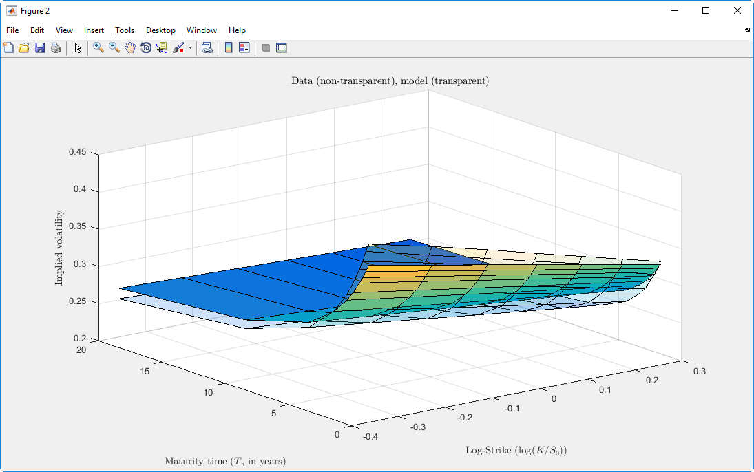
cloudendThe image below shows the model surface graph that is generated during the computational Project. This graph is updated automatically whenever new intermediate result data has been received from Job #1.
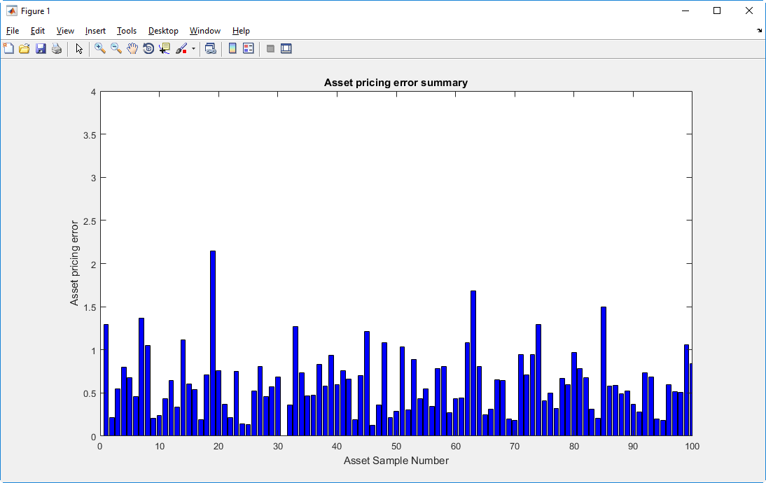
The image below shows the summary graph that is generated when the code is executed. Each bar in the graph is updated automatically as new intermediate result data is received from a Job
1.5. Accessing Results
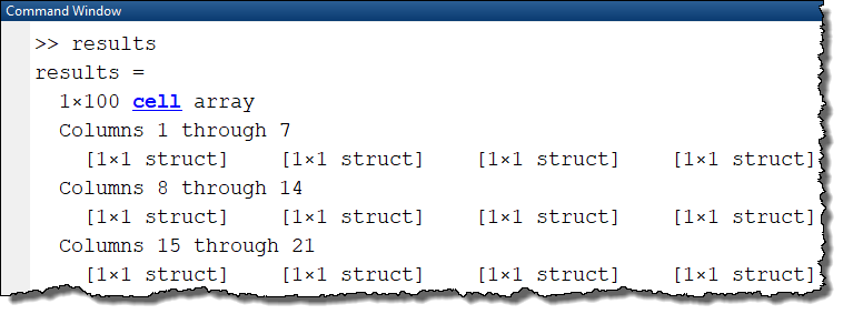
Accessing the computational results in the local and distributed versions can be done in an identical manner: by accessing the results workspace variable, which will be a 1x100 cell array.
The screen capture below illustrates how the results can be accessed after completing the computations in Techila Distributed Computing Engine.
As the results are available in identical format, this means that any result post-processing could be done using identical code. This in turn reduces the amount of code changes required and makes integrating the distributed version in to an existing process flow easier.