1. MATLAB - Value-at-Risk Calculation
This example illustrates how to use Techila Distributed Computing Engine to speed up Value-at-Risk computations implemented with MATLAB.
The information on this page is intended to supplement the information in the original paper discussing this application. You can download the paper using the link shown below:
In addition to the performance statistics available in paper above, additional testing was also done in order to measure how well the use-case scales performance-wise when more computing power is used. In short, an acceleration of 610x was achieved, reducing the wallclock time of an 11 hour computation to just 65 seconds. More information can be found in Performance Summary.
1.1. Introduction
One of the most common risk measures in the finance industry is Value-at-Risk (VaR). Value-at-Risk measures the amount of potential loss that could happen in a portfolio of investments over a given time period with a certain confidence interval. It is possible to calculate VaR in many different ways, each with their own pros and cons. Monte Carlo simulation is a popular method and is used in this example.
In the simplified VaR model used in the example, the value of a portfolio of financial instruments is simulated under a set of economic scenarios. The set of financial instruments in this example is limited to a set of fixed coupon bonds and equity options. The scenarios can be analyzed independently, meaning that the computations can be sped up significantly by analyzing the scenarios simultaneously on a large number of Techila Worker nodes.
This example is available for download at the following link:
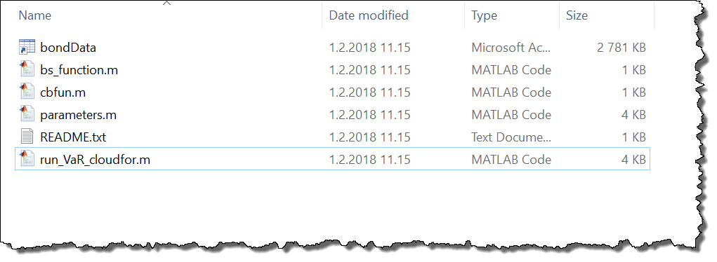
The contents of the zip file is shown below for reference:
1.2. Data Locations & Management
This example uses a set of pre-generated bond data, which is stored in a file called bondData.mat. This file is included in the zip-file, as can be seen from the previous screenshot.
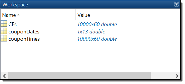
The contents of this file is loaded to the local MATLAB workspace, which creates variables named CFs, couponDates and couponTimes.
The data stored in variables CFs and couponTimes will be used when analyzing the scenarios. When processing the scenarios locally, the values of variables needed in the computations will be read from the local workspace, as in any other standard MATLAB application. In the distributed version of this application, variables will be automatically transferred to Techila Workers participating in the computations.
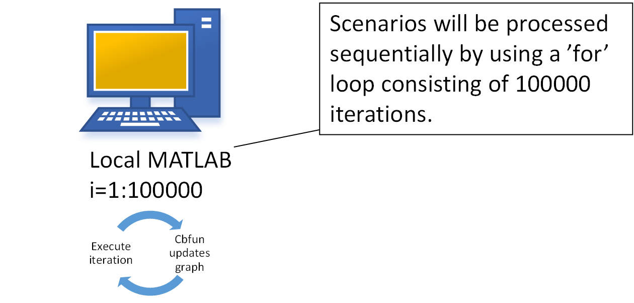
1.3. Sequential Local Processing
The computations could be executed locally by using a for loop structure shown below. Please note that the code package does not include a locally executable version, but the cloudfor version can be easily modified into a local for version as shown in the code snippet below.
for i = 1:nrOfScenarios
    % Apply scenario on the interest rate curve
    PCAshock = scenarios(i,1)*PCA1+scenarios(i,2)*PCA2+scenarios(i,3)*PCA3;
    rateShock = exp(interp1(PCA.t,PCAshock,ir.t,'spline'));
    shockedRate = ((ir.r+ir.displacement) .* rateShock) - ir.displacement;

    % Option valuation under the different scenarios
    rate = interp1(ir.t,shockedRate,option.Maturity,'linear');
    vol = interp2(iv.t,iv.M,(scenarios(i,5)-1*volshock.surface)+1,option.Maturity,max(min(S0*scenarios(i,4)./K,max(iv.M)),min(iv.M)));
    p_options = bs_function(S0*scenarios(i,4),K,option.Maturity,rate,vol,isCall)';

    % Bond valuation under the different scenarios
    rate = interp1(ir.t,shockedRate,couponTimes,'linear');
    p_bonds = sum(CFs.*exp(-couponTimes.*rate/100),2,'omitnan');

    % Return the result
    portfolioValue(i) = [p_options;p_bonds]'*pos;

    % Visualize the results
    cbfun(portfolioValue,basePortfolioValue))
end
Each iteration stores the computational result in the portfolioValue. Each iteration is independent, meaning there are no recursive dependencies. The results are visualized by performing a cbfun call, which updates the figure with new scenario data.
1.4. Distributed Processing
The code below shows the cloudfor version of the code, which will perform the computations in Techila Distributed Computing Engine. The syntax shown below will essentially push all code between the cloudfor and cloudend keywords to Techila Distributed Computing Engine where it will be executed on Techila Workers.
All parameters that start with %cloudfor are optional control parameter used to fine tune the behaviour of the computations. The effect of the control parameters is illustrated in the image below. For more information about the cloudfor helper function, please see Techila Distributed Computing Engine with MATLAB.
More information about the used control parameters can also be found in the source code comments.
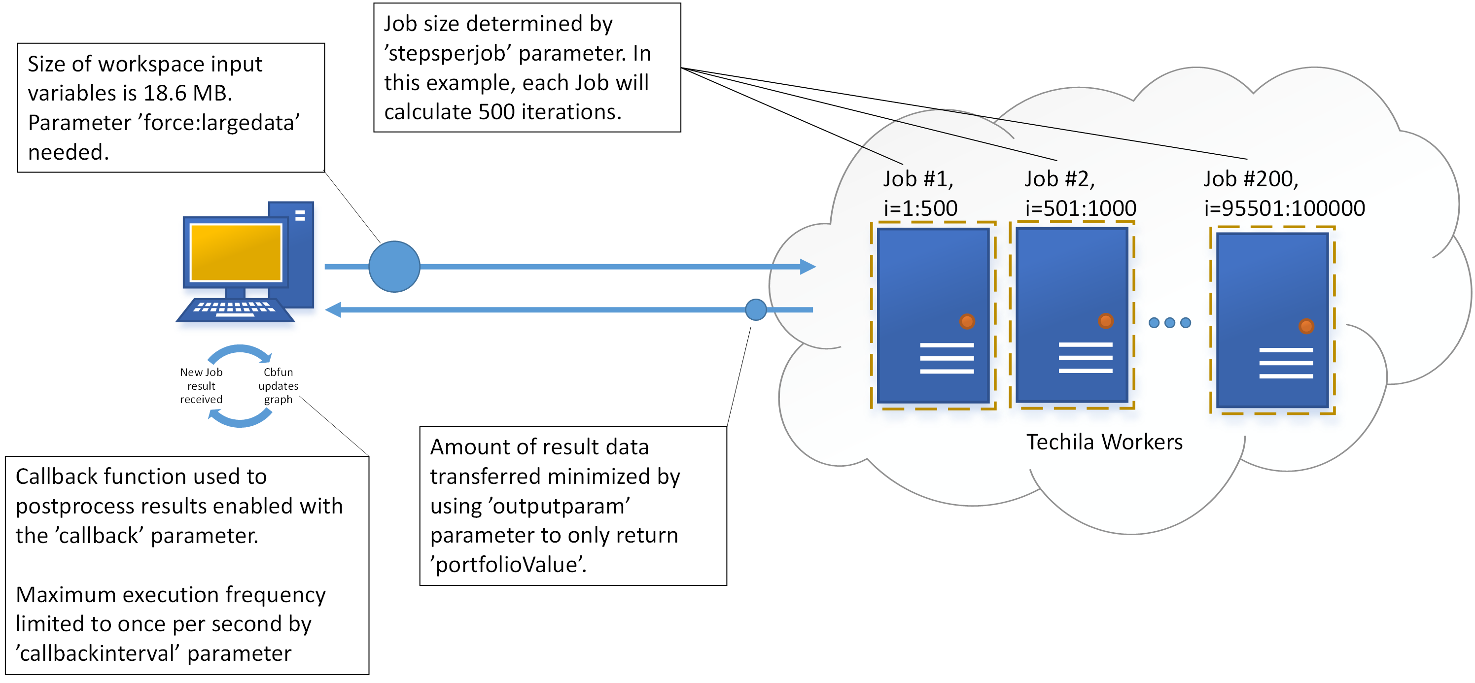
% How many iterations per Job
itersinjob = 500;

cloudfor i = 1:nrOfScenarios
%cloudfor('stepsperjob',itersinjob)
%cloudfor('callback','cbfun(portfolioValue,basePortfolioValue)')
%cloudfor('force:largedata')
%cloudfor('outputparam',portfolioValue)
%cloudfor('callbackinterval','1s')
    if isdeployed
    % Apply scenario on the interest rate curve
    PCAshock = scenarios(i,1)*PCA1+scenarios(i,2)*PCA2+scenarios(i,3)*PCA3;
    rateShock = exp(interp1(PCA.t,PCAshock,ir.t,'spline'));
    shockedRate = ((ir.r+ir.displacement) .* rateShock) - ir.displacement;

    % Option valuation under the different scenarios
    rate = interp1(ir.t,shockedRate,option.Maturity,'linear');
    vol = interp2(iv.t,iv.M,(scenarios(i,5)-1*volshock.surface)+1,option.Maturity,max(min(S0*scenarios(i,4)./K,max(iv.M)),min(iv.M)));
    p_options = bs_function(S0*scenarios(i,4),K,option.Maturity,rate,vol,isCall)';

    % Bond valuation under the different scenarios
    rate = interp1(ir.t,shockedRate,couponTimes,'linear');
    p_bonds = sum(CFs.*exp(-couponTimes.*rate/100),2,'omitnan');

    % Return the result
    portfolioValue(i) = [p_options;p_bonds]'*pos;
    end
cloudend
1.5. Result Postprocessing
The result data post processing consists of plotting a histogram and calculating the quantiles. The figure containing the post processed data is shown below for reference.
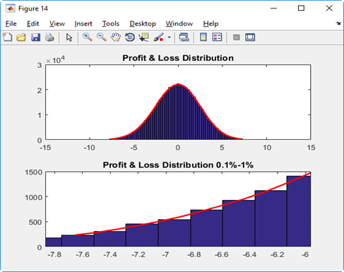
When using cloudfor, any result variables received from the Techila Workers will be automatically imported to the MATLAB workspace on the end-users computer. This means that after completing the cloudfor loop, all result data will be available in an identical format (same sizes, same data types) as in the local version. This in turn means that the code used to for post processing will be identical in both the local and distributed versions of the applications.
% Plot histogram and calculate quantiles
probs = [0.001,0.005,0.01,0.1,0.25,0.5,0.75,0.9,0.99,0.995,0.999];
quantiles = quantile(100*(portfolioValue/basePortfolioValue-1), probs);
disp('Quantiles:')
disp(probs)
disp(quantiles)
subplot(2,1,1), histfit(100*(portfolioValue/basePortfolioValue-1),100,'kernel');
title('Profit & Loss Distribution')
subplot(2,1,2), histfit(100*(portfolioValue/basePortfolioValue-1),100,'kernel');
title('Profit and Loss Distribution 0.1-1% percentile')
xlim([quantile(100*(portfolioValue/basePortfolioValue-1),0.001) quantile(100*(portfolioValue/basePortfolioValue-1),0.01)])
1.6. Performance Summary
The test case was executed using Techila in Google Cloud Launcher. Instructions for setting up your own Techila Distributed Computing Engine environment can be found in Techila Distributed Computing Engine in Google Cloud Platform Marketplace.
The test case consisted of analyzing a total 614400 scenarios (nrOfScenarios = 614400; in parameters.m).
The table below shows the wall clock times and acceleration factors achieved when increasing the amount of CPU cores used to solve 614400 scenarios. Computations were done using n1-standard-4 instances.
| CPU Core Count | Wallclock Time |
|---|---|
1 |
11 hours 1 minute 2 seconds |
4 |
2 hours 52 minutes |
16 |
43 minutes 33 seconds |
32 |
22 minutes 33 seconds |
64 |
11 minutes 28 seconds |
128 |
5 minutes 58 seconds |
160 |
4 minutes 54 seconds |
256 |
3 minutes 12 seconds |
512 |
1 minutes 59 seconds |
1024 |
1 minute 5 seconds |