MATLAB - Parallelizing Fminsearch Optimization Routines

1. Introduction

Numerical optimization has a central role in many fields of applied mathematics ranging from quantitative finance to control theory. In situations, where the optimization process uses a computationally intensive, parallelizable loss function, Techila Distributed Computing Engine (TDCE) can be used to improve the performance by processing the independent subtasks simultaneously on multiple Techila Workers.

This document shows, how the use of distributed computing can improve a user’s productivity, and how TDCE can maximize the cost efficiency of the entire computing workflow from the development to the use of a computing infrastructure.

The code examples presented in this document illustrate how to use TDCE to speed up the fminsearch optimization routines, used in an option pricing model. The code is written in MATLAB.

The information in this document is intended to supplement the information in the original paper, which can be downloaded from the link shown below:

View paper

The code material presented in this document is available for download at the following link:

Fminsearch code package

2. Code Overview

The following chapters contain short walkthroughs of the three different code samples referred to in this paper. The terms used to refer to these code samples are "Local", "Approach A" and "Approach B", following the terminology used in the paper.

The image below illustrates the directory structure of the code package after it has been extracted to a computer.

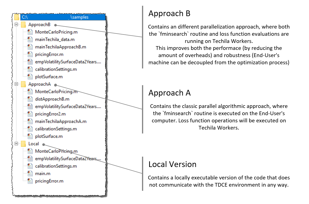
Figure 1. Each folder contains a different version of the same model pricing algorithm.

2.1. Local Version

Should you be interested in running the code on your own PC, without TDCE, a locally executable version of the application can be found in the Local directory. The local version can be executed by running the main.m file, which will start the fminsearch routine on the End-User’s computer.

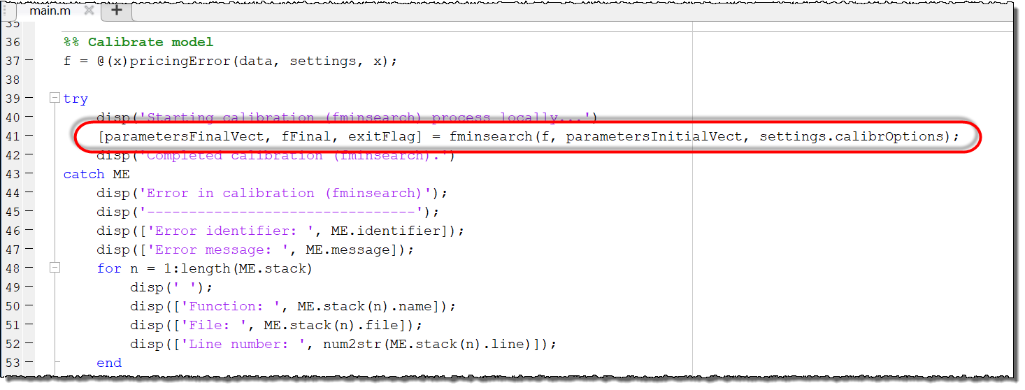
Figure 2. The highlighted code line in main.m will run the entire fminsearch routine locally on the End-User’s computer. This includes the computationally intensive operations of the loss functions.

The loss function contains a Monte Carlo routine, where the variable settings.nSim determines the number of simulations to be performed. Each simulation is independent of other simulations, meaning they can be executed simultaneously in the distributed versions (Approach A and Approach B).

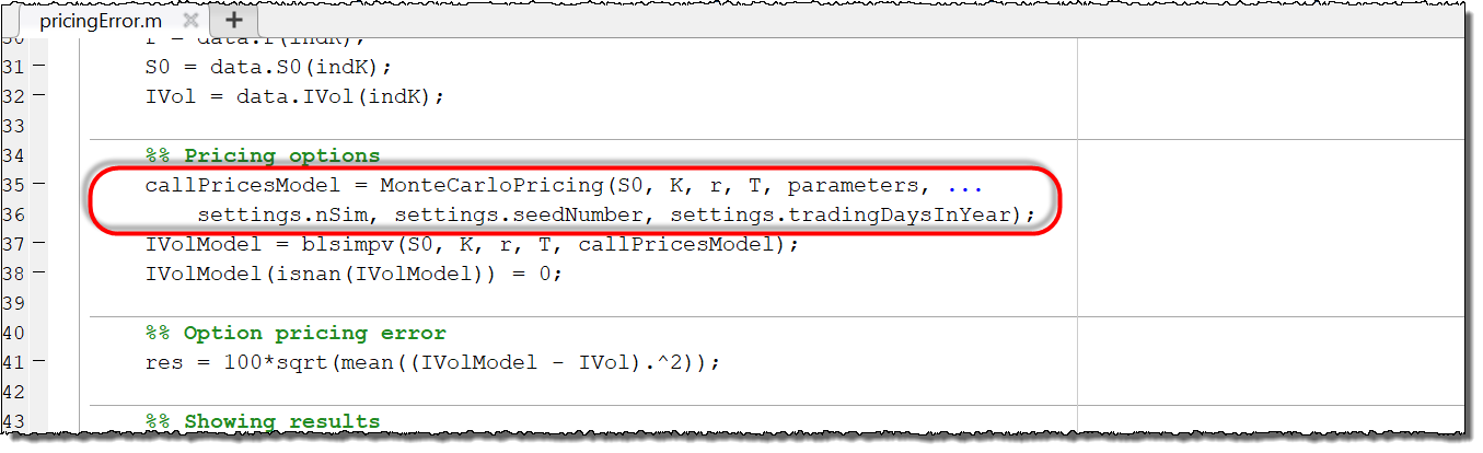
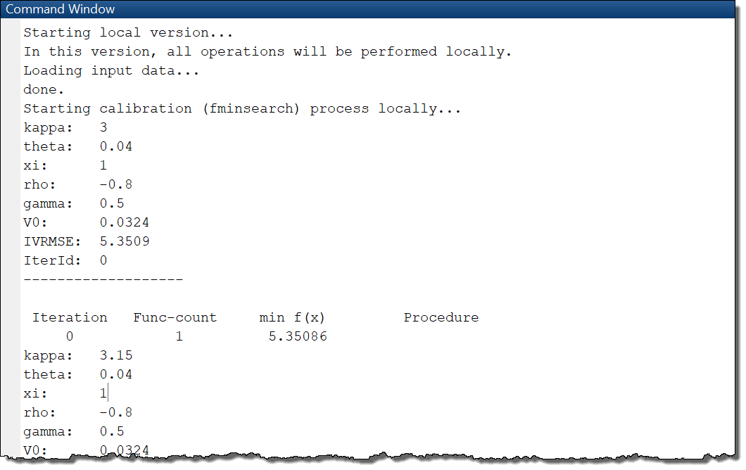
Figure 3. The highlighted code line in pricingError.m will start the computationally intensive Monte Carlo operations locally, on the End-User’s computer.

As the fminsearch optimization process advances, information about parameter values will be printed to the command window.

Figure 4. Progress information about the optimization process.

2.2. Approach A

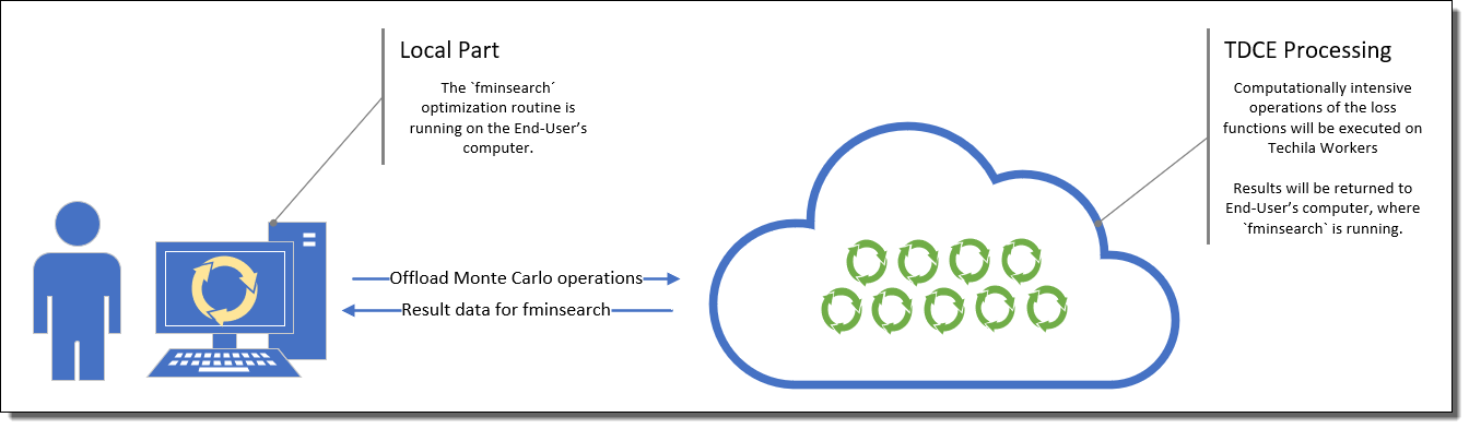
The code material for the Approach A uses distributed computing. This version of the application is located in the ApproachA directory. This version can be executed by running the mainTechilaApproachA.m file. In this version, the fminsearch routine will still run on the End-User’s computer, similarly as in the local version described above.

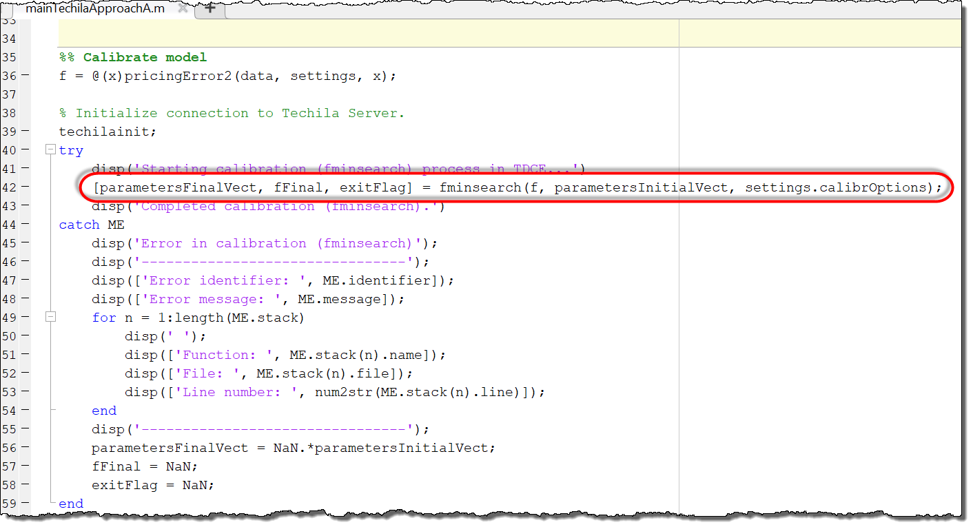
Figure 5. The fminsearch routine is located in the mainTechilaApproachA.m file, which will be executed locally.

The difference between the Local version and Approach A is that, in the MonteCarloPricing.m file of Approach A, a cloudfor loop has been used to parallelize the computationally intensive Monte Carlo operations.

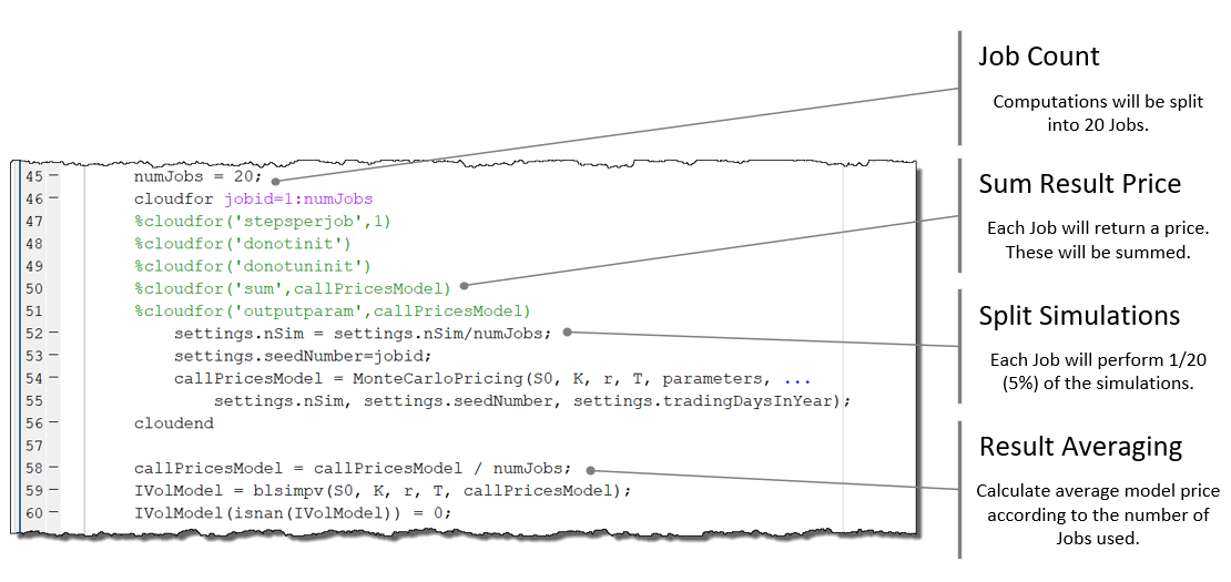
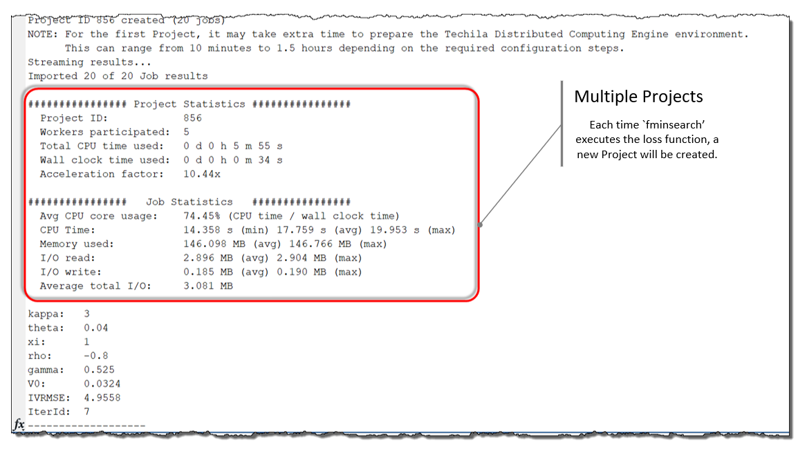
Figure 6. Monte Carlo simulations are independent, meaning the simulations can be divided into smaller subsets and processed simultaneously in TDCE.

As the cloudfor loop is located inside the loss function, a new computational Project will be created every time the fminsearch executes the loss function. These computational Projects will be used to process the computationally intensive Monte Carlo operations of the loss function.

Figure 7. The fminsearch routine runs on the End-User’s computer, meaning overheads related to initializing the distributed computing environment will be incurred every time the loss function is executed.

Project statistics and information about the parameters will be displayed each time a new Project has been completed.

Figure 8. Project statistics will be automatically displayed every time a Project is completed.

2.3. Approach B

In this version, both the fminsearch routine and all operations of the loss functions will be offloaded to the TDCE environment. The End-User’s computer will only be used to run a cloudfor loop, which will create the Project.

Figure 9. The cloudfor loop is located in the mainTechilaApproachB.m file, which will be executed locally. All operations related to the optimization process will run in the TDCE environment, not on the End-User’s computer

The above cloudfor loop will perform two different types of operations in Jobs:

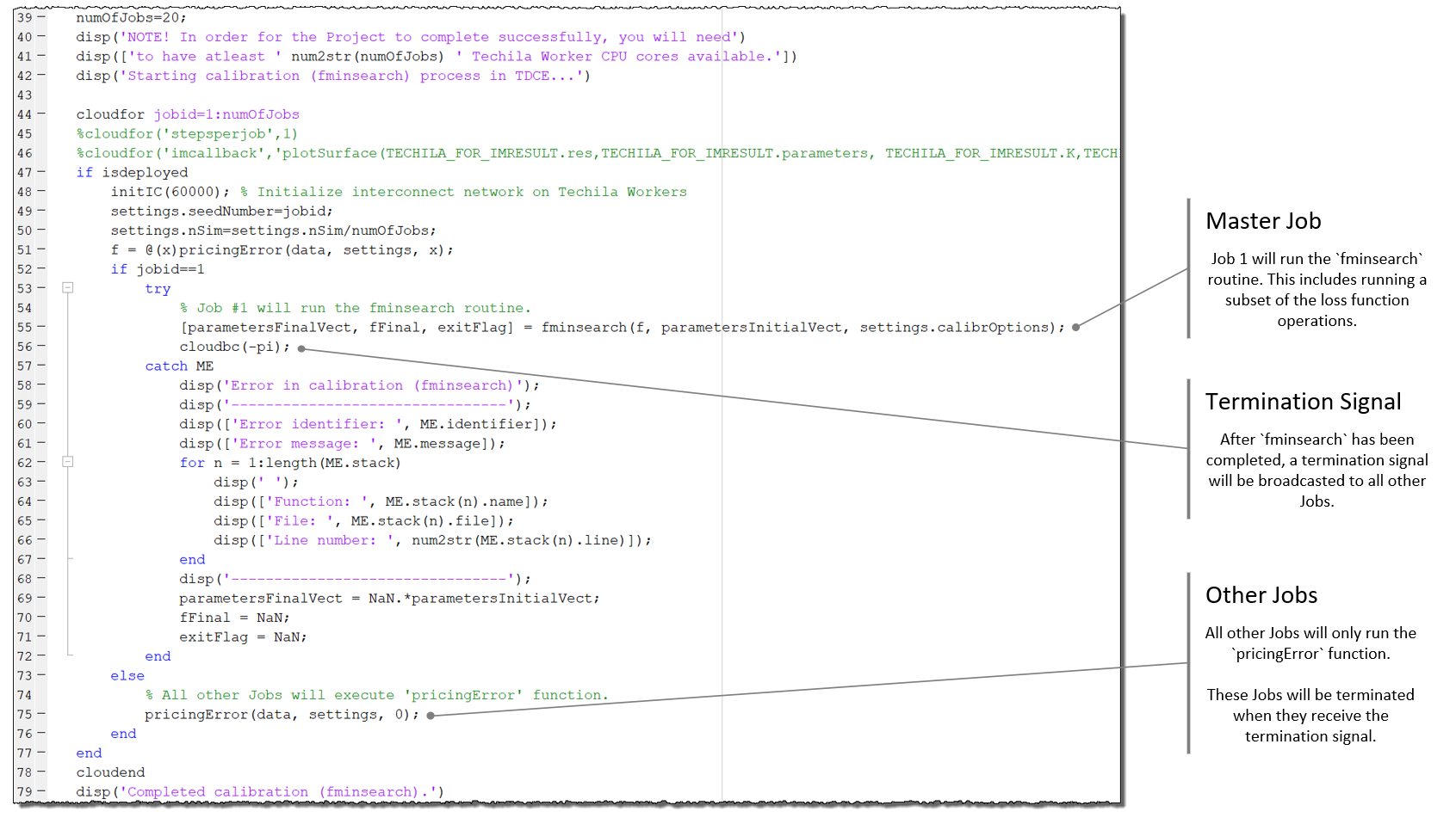
Job 1: Will run the fminsearch routine and the computationally intensive Monte Carlo operations of the loss functions. This Job will also transfer data with other Jobs (2-20) using the Techila Interconnect feature.
Jobs 2-20: Will only run the computationally intensive Monte Carlo operations of the loss functions. Will transfer data with Job 1 using the Techila Interconnect feature.

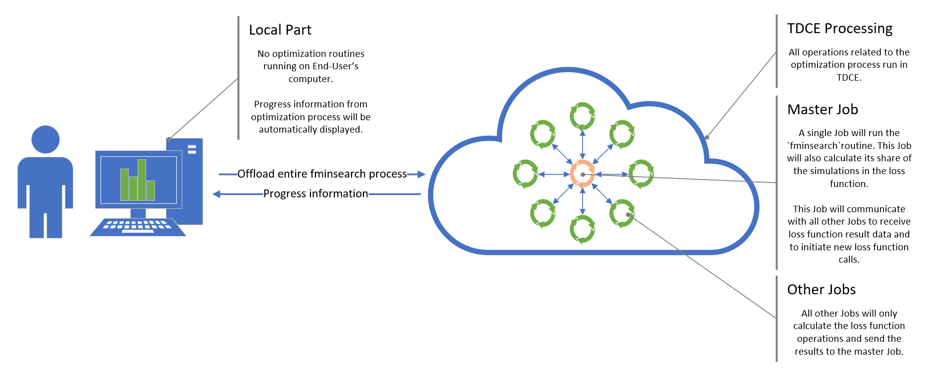
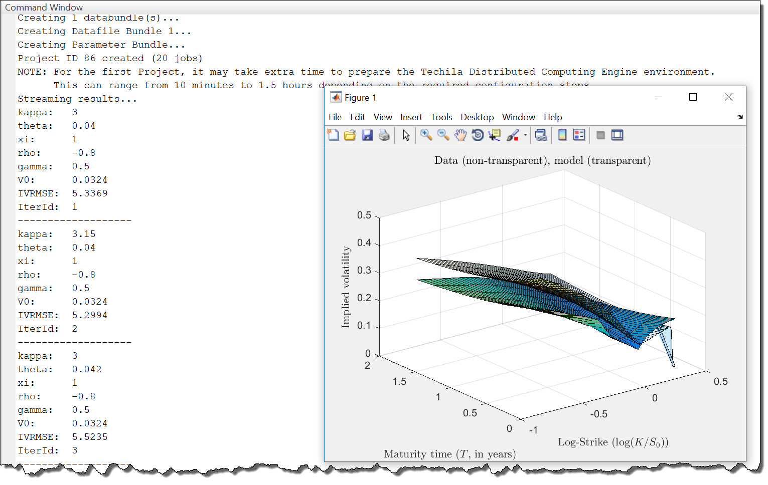
Figure 10. The computational Project will consist of two types of Jobs: one master Job running fminsearch and all other Jobs only running the computationally intensive loss function operations.

As the cloudfor loop was used to offload the entire optimization process, only one computational Project will be created. Progress information about the optimization process will be automatically returned to the End-User’s computer, where it will be displayed in the MATLAB command window.

Figure 11. Progress information a model data visualization will be automatically displayed on the End-User’s computer.

3. Performance

The paper describes the performance of these three different approaches when doing the test run consisting of 507 optimization iterations.

The experiments show how the use of distributed computing can improve a user’s productivity, and how cloudfor can maximize the cost efficiency of computing:

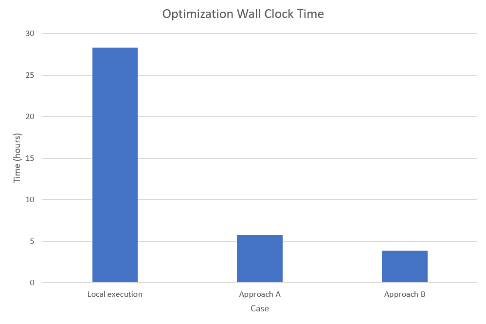
It is possible to cut down the wall-clock time clearly by the use of distributed computing: Approach A reduces wall-clock time by 80% in contrast to the local experiment that did not use distributed computing. Respectively, Approach B reduces wall-clock time by 86% in contrast to the local experiment. The time saved translates directly into more productivity.
In the terms of wall-clock time used, Approach B is 33% more efficient than Approach A. This makes Approach B considerably higher value when using distributed computing, especially in a cloud-based infrastructures where the user pays per use. The Approach B demonstrates that, by minimizing the overhead caused by i) information transfer between the end-user workstation and cloud and ii) iterative initializations and finalizations of computing nodes, we can save one third of wall-clock time and maximize the cost efficiency of our infrastructure usage.

The calibration times of the three experiments are described below for reference. The full data can be found in the paper.

	Wall-clock time	CPU time
No distribution	1d04h18m	1d04h12m
Approach A	5h44m	1d16h43m
Approach B	3h51m	1d04h49m

Wall-clock time

CPU time

No distribution

1d04h18m

1d04h12m

Approach A

5h44m

1d16h43m

Approach B

3h51m

1d04h49m

A graphical visualization of the performance data is shown below.

Figure 12. Performance of different approaches.